Aggregating and Analyzing Data with dplyr
Overview
Teaching: 60 min
Exercises: 15 minQuestions
How can I manipulate dataframes without repeating myself?
Objectives
Select certain columns in a data frame with the
dplyrfunctionselect.Extract certain rows in a data frame according to logical (boolean) conditions with the
dplyrfunctionfilter.Link the output of one
dplyrfunction to the input of another function with the ‘pipe’ operator%>%.Add new columns to a data frame that are functions of existing columns with
mutate.Use the split-apply-combine concept for data analysis.
Use
summarize,group_by, andcountto split a data frame into groups of observations, apply summary statistics for each group, and then combine the results.Employ the ‘split-apply-combine’ concept to split the data into groups, apply analysis to each group, and combine the results.
Export a data frame to a .csv file.
Data manipulation using dplyr and tidyr from tidyverse package
Bracket subsetting is handy, but it can be cumbersome and difficult to read,
especially for complicated operations. Enter dplyr. dplyr is a package for
making tabular data manipulation easier. It pairs nicely with tidyr which enables you to swiftly convert between different data formats for plotting and analysis.
The tidyverse package is an “umbrella-package” that installs tidyr, dplyr, and several other packages useful for data analysis, such as ggplot2, tibble, etc.
The tidyverse package tries to address 3 common issues that arise when
doing data analysis with some of the functions that come with R:
- The results from a base R function sometimes depend on the type of data.
- Using R expressions in a non standard way, which can be confusing for new learners.
- Hidden arguments, having default operations that new learners are not aware of.
First we have to make sure we have the tidyverse package (including dplyr
and tidyr) installed.
Install tidyverse
ON NOTABLE RSTUDIO SERVER:
If you’re using the EDINA Notable RStudio Server, tidyverse is already installed,
so you can skip this step. It’s worth knowing how to install a package for future
though, so check out the instructions for locally-installed RStudio.
ON LOCAL RSTUDIO:
Install the package you want by using the install.package() function, with the
name of the package you want inside the brackets, within quotes.
If you get an error, make sure you’ve spelled the package name correctly.
install.packages("tidyverse") ## install tidyverse
You might get asked to choose a CRAN mirror – this is asking you to choose a site to download the package from. The choice doesn’t matter too much; I’d recommend choosing the RStudio mirror.
Load tidyverse package
To load the package (whether in Notable or running RStudio locally), type (without quotes this time!):
## load the tidyverse packages, incl. dplyr
library(tidyverse)
Warning: package 'tidyverse' was built under R version 4.0.2
Error: package or namespace load failed for 'tidyverse' in dyn.load(file, DLLpath = DLLpath, ...):
 unable to load shared object '/Library/Frameworks/R.framework/Versions/4.0/Resources/library/Rcpp/libs/Rcpp.so':
  dlopen(/Library/Frameworks/R.framework/Versions/4.0/Resources/library/Rcpp/libs/Rcpp.so, 6): Symbol not found: _EXTPTR_PTR
  Referenced from: /Library/Frameworks/R.framework/Versions/4.0/Resources/library/Rcpp/libs/Rcpp.so
  Expected in: /Library/Frameworks/R.framework/Versions/4.0/Resources/lib/libR.dylib
 in /Library/Frameworks/R.framework/Versions/4.0/Resources/library/Rcpp/libs/Rcpp.so
You only need to install a package once per computer, but you need to load it every time you open a new R session and want to use that package.
What are dplyr and tidyr?
The package dplyr provides easy tools for the most common data manipulation
tasks. It is built to work directly with data frames, with many common tasks
optimized by being written in a compiled language (C++). An additional feature is the
ability to work directly with data stored in an external database. The benefits of
doing this are that the data can be managed natively in a relational database,
queries can be conducted on that database, and only the results of the query are
returned.
This addresses a common problem with R in that all operations are conducted in-memory and thus the amount of data you can work with is limited by available memory. The database connections essentially remove that limitation in that you can connect to a database of many hundreds of GB, conduct queries on it directly, and pull back into R only what you need for analysis.
The package tidyr addresses the common problem of wanting to reshape your data for
plotting and use by different R functions. Sometimes we want data sets where we have one
row per measurement. Sometimes we want a data frame where each measurement type has its
own column, and rows are instead more aggregated groups
(e.g., a time period, an experimental unit like a plot or a batch number).
Moving back and forth between these formats is non-trivial, and tidyr gives you tools
for this and more sophisticated data manipulation.
To learn more about dplyr and tidyr after the workshop, you may want to check out this
handy data transformation with dplyr cheatsheet
and this one about tidyr.
As before, we’ll read in our variants data:
variants <- read.csv("https://ndownloader.figshare.com/files/14632895")
We then want to check our variants object:
## inspect the data
str(variants)
## preview the data
view(variants)
Next, we’re going to learn some of the most common dplyr functions as well
as using pipes to combine them:
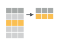
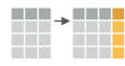
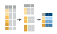
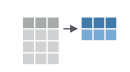
If we think about our data as rectangular, these illustrations from the dplyr data transformation cheatsheet help us understand how they manupulate the data frame.
select(): subset columns

filter(): subset rows on conditions
mutate(): create new columns by using information from other columns
group_by()andsummarize(): create summary statistics on grouped data
count(): count discrete values

Selecting columns and filtering rows
Using bracket notation, in order to pull out certain columns, we would have to know which index referred to that column, which took an extra step, and if we had re-ordered our columns or added one in the middle, the indexes in our script would suddenly refer to the ‘wrong’ column, which might cause confusion!
As a refresher, here’s how we pulled out columns using the bracket notation:
# get columns: sample_id, REF, ALT, DP
variants[, c(1, 5, 6, 12)]
   sample_id      REF       ALT DP
1 SRR2584863        T         G  4
2 SRR2584863        G         T  6
3 SRR2584863        G         T 10
4 SRR2584863 CTTTTTTT CTTTTTTTT 12
5 SRR2584863     CCGC    CCGCGC 10
6 SRR2584863        C         T 10
But our code isn’t very easy to understand and we’d need to see the output to make sure we had the correct columns.
Enter dplyr!
How to select() columns
To select columns of a data frame, use select(). The first argument to this
function is the data frame (variants), and the subsequent arguments are the
columns to keep.
select(variants, sample_id, REF, ALT, DP)
Error in select(variants, sample_id, REF, ALT, DP) %>% head(): could not find function "%>%"
This code is much easier to understand!
To select all columns except certain ones, put a “-“ in front of the variable to exclude it.
select(variants, -CHROM)
Error in select(variants, -CHROM) %>% head(): could not find function "%>%"
Tibbles and as_tibble()
One thing we still have is an issue with how our output prints - it takes up a
lot of space in our console, and it’s a little confusing to read. We might get
a warning like [ reached 'max' / getOption("max.print") -- omitted 551 rows ]
if we’re showing too many rows. We might usually just want to view the first few
rows to check our output makes sense, not the first few hundred!
Luckily, the tidyverse has another package to help us: tibble.
Using the function as_tibble() will convert our data.frame object into the
slightly friendlier "tibble" format, which is officially known as a tbl_df.
Tibbles have better formatting and printing and stricter handling of data types,
and are the ‘central data structure’ for the tidyverse set of packages.
They also help make our data manipulation much easier!
We use our variants data frame as the argument
variants <- as_tibble(variants)
select(variants, sample_id, REF, ALT, DP)
Error in as_tibble(variants): could not find function "as_tibble"
Error in select(variants, sample_id, REF, ALT, DP): could not find function "select"
This looks much better!
How to filter() rows
To choose rows, use filter():
filter(variants, sample_id == "SRR2584863")
Error in filter(variants, sample_id == "SRR2584863"): object 'sample_id' not found
Note that this is equivalent to the base R code below, but is easier to read!
variants[variants$sample_id == "SRR2584863",]
Pipes
But what if you wanted to select and filter? We can do this with pipes.
Pipes let you take the output of one function and send it directly to the next, which is useful when you need to many things to the same data set. It was possible to do this before pipes were added to R, but it was much messier and more difficult.
Pipes in R look like %>% and are made available via the magrittr package,
which is installed as part of dplyr. If you use RStudio, you can type the pipe
with Ctrl + Shift + M if you’re using a PC,
or Cmd + Shift + M if you’re using a Mac.
variants %>%
  filter(sample_id == "SRR2584863") %>%
  select(REF, ALT, DP)
Error in variants %>% filter(sample_id == "SRR2584863") %>% select(REF, : could not find function "%>%"
In the above code, we use the pipe to send the variants dataset first through
filter(), to keep rows where sample_id matches a particular sample, and then
through select() to keep only the REF, ALT, and DP columns. Since %>%
takes the object on its left and passes it as the first argument to the function
on its right, we don’t need to explicitly include the data frame as an argument
to the filter() and select() functions any more.
Some may find it helpful to read the pipe like the word “then”. For instance,
in the above example, we took the data frame variants, then we filtered
for rows where sample_id was SRR2584863, then we selected the REF, ALT,
and DP columns, then we showed only the first six rows.
The dplyr functions by themselves are somewhat simple,
but by combining them into linear workflows with the pipe, we can accomplish
more complex manipulations of data frames.
NOTE: Pipes work with non-dplyr functions, too, as long as the dplyr or magrittr package is loaded.
If we want to create a new object with this smaller version of the data we can do so by assigning it a new name:
SRR2584863_variants <- variants %>%
  filter(sample_id == "SRR2584863") %>%
  select(REF, ALT, DP)
Error in variants %>% filter(sample_id == "SRR2584863") %>% select(REF, : could not find function "%>%"
This new object includes all of the data from this sample. Let’s look at just the first six rows to confirm it’s what we want:
head(SRR2584863_variants)
Error in head(SRR2584863_variants): object 'SRR2584863_variants' not found
Exercise: Pipe and filter
Starting with the
variantsdataframe, use pipes to subset the data to include only observations from SRR2584863 sample, where the filtered depth (DP) is at least 10. Retain only the columnsREF,ALT, andPOS.Solution
 variants %>%
 filter(sample_id == "SRR2584863" & DP >= 10) %>%
 select(REF, ALT, POS)
Error in variants %>% filter(sample_id == "SRR2584863" & DP >= 10) %>% : could not find function "%>%"
Mutate
Frequently you’ll want to create new columns based on the values in existing
columns, for example to do unit conversions or find the ratio of values in two
columns. For this we’ll use the dplyr function mutate().
We have a column titled “QUAL”. This is a Phred-scaled confidence score that a polymorphism exists at this position given the sequencing data. Lower QUAL scores indicate low probability of a polymorphism existing at that site. We can convert the confidence value QUAL to a probability value according to the formula:
Probability = 1- 10 ^ -(QUAL/10)
Let’s add a column (POLPROB) to our variants dataframe that shows
the probability of a polymorphism at that site given the data.
variants %>%
  mutate(POLPROB = 1 - (10 ^ -(QUAL/10))) %>%
  glimpse()
Error in variants %>% mutate(POLPROB = 1 - (10^-(QUAL/10))) %>% glimpse(): could not find function "%>%"
NOTE: We’ve used the glimpse() function to show only the first few
values of data for each variable - you can see it’s quite similar to
str() in how it shows the output. You could also use head() in the same way
to just show 6 rows rather than the 10 rows shown by default with tibbles.
Exercise
There are a lot of columns in our dataset, so let’s just look at the
sample_id,POS,QUAL, andPOLPROBcolumns for now. Add a line to the above code to only show those columns and show the output viaglimpse().Solution
variants %>%
mutate(POLPROB = 1 - 10 ^ -(QUAL/10)) %>%
select(sample_id, POS, QUAL, POLPROB) %>%
glimpse()
Error in variants %>% mutate(POLPROB = 1 - 10^-(QUAL/10)) %>% select(sample_id, : could not find function "%>%"
Split-apply-combine data analysis and the summarize() function
Many data analysis tasks can be approached using the “split-apply-combine”
paradigm: split the data into groups, apply some analysis to each group, and
then combine the results. dplyr makes this very easy through the use of the
group_by() function, which splits the data into groups.
The summarize() function
group_by() is often used together with summarize(), which collapses each
group into a single-row summary of that group. group_by() takes as arguments
the column names that contain the categorical variables for which you want
to calculate the summary statistics.
For example, if we wanted to group by sample_id and find the number of rows
of data for each sample, we would do:
variants %>%
  group_by(sample_id) %>%
  summarize(n_observations = n())
Error in variants %>% group_by(sample_id) %>% summarize(n_observations = n()): could not find function "%>%"
Here the summary function used was n() to find the count for each
group, which we displayed in a column which we called n_observations.
We can also apply many other functions to individual columns
to get other summary statistics. For example, we can use built-in functions like
mean(), median(), min(), and max(). These are called “built-in
functions” because they come with R and don’t require that you install any
additional packages.
So to view the highest filtered depth (DP) for each sample:
variants %>%
  group_by(sample_id) %>%
  summarize(max(DP))
Error in variants %>% group_by(sample_id) %>% summarize(max(DP)): could not find function "%>%"
Handling Missing Values In Data
By default, all R functions operating on vectors that contains missing data will return NA.
It’s a way to make sure that users know they have missing
data, and make a conscious decision on how to deal with it. When
dealing with simple statistics like the mean, the easiest way to
ignore NA (the missing data) is to use na.rm = TRUE (rm stands for
remove).
When working with data frames (and tibbles!), we have slightly more options.
Exporting data
Now that you have learned how to use dplyr to extract information from
or summarize your raw data, you may want to export these new data sets to share
them with your collaborators or for archival.
Similar to the read.csv() function used for reading CSV files into R, there is
a write.csv() function that generates CSV files from data frames.
Before using write.csv(), we should preferrably create a new folder, data,
in our working directory that will store this generated dataset. We don’t want
to write generated datasets in the same directory as our raw data. It’s good
practice to keep them separate.
Ideally, we should have a data_raw folder should only contain the raw, unaltered data, and should be left alone to make sure we don’t delete or modify it. In contrast,
our script will generate the contents of the data directory, so even if the
files it contains are deleted, we can always re-generate them.
In preparation for our next lesson on plotting, we are going to prepare a cleaned up version of the data set that doesn’t include any missing data.
Much of this lesson was copied or adapted from Jeff Hollister’s materials
Key Points
Use the
dplyrpackage to manipulate dataframes.Use
select()to choose variables from a dataframe.Use
filter()to choose data based on values.Use
group_by()andsummarize()to work with subsets of data.Use
mutate()to create new variables.