Starting With Data
Overview
Teaching: 30 min
Exercises: 30 minQuestions
How can I import data in Python?
What is Pandas?
Why should I use Pandas to work with data?
Objectives
Navigate the workshop directory and download a dataset.
Explain what a library is and what libraries are used for.
Describe what the Python Data Analysis Library (Pandas) is.
Load the Python Data Analysis Library (Pandas).
Read tabular data into Python using Pandas.
Describe what a DataFrame is in Python.
Access and summarize data stored in a DataFrame.
Define indexing as it relates to data structures.
Perform basic mathematical operations and summary statistics on data in a Pandas DataFrame.
Create simple plots.
Working With Pandas DataFrames in Python
We can automate the process of performing data manipulations in Python. It’s efficient to spend time building the code to perform these tasks because once it’s built, we can use it over and over on different datasets that use a similar format. This makes our methods easily reproducible. We can also easily share our code with colleagues and they can replicate the same analysis.
Starting in the same spot
To help the lesson run smoothly, let’s ensure everyone is in the same directory. This should help us avoid path and file name issues. At this time please navigate to the workshop directory. If you are working in Jupyter Notebook be sure that you start your notebook in the workshop directory.
A quick aside that there are Python libraries like OS Library that can work with our directory structure, however, that is not our focus today.
Our Data
We are studying ocean waves and temperature in the seas around the UK.
For this lesson we will be using a subset of data from Centre for Environment Fisheries and Aquaculture Science (Cefas). WaveNet, Cefas’ strategic wave monitoring network for the United Kingdom, provides a single source of real-time wave data from a network of wave buoys located in areas at risk from flooding. https://wavenet.cefas.co.uk/
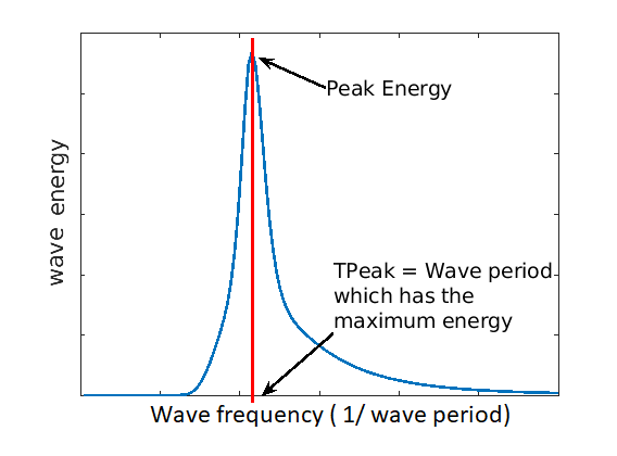
If we look out to sea, we notice that waves on the sea surface are not simple sinusoids. The surface appears to be composed of random waves of various lengths and periods. How can we describe this complex surface?
By making some simplifications and assumptions, we fit an idealised ‘spectrum’ to describe all the energy held in different wave frequencies. This describes the wave energy at a point, covering the energy in small ripples (high frequency) to long period (low frequency) swell waves. This figure shows an example idealised spectrum, with the highest energy around wave periods of 11 seconds.
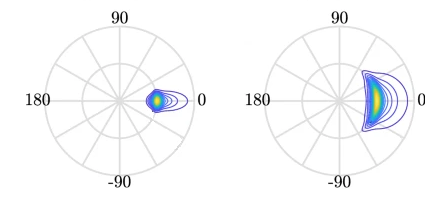
We can go a step further, and also associate a wave direction with the amount of energy. These simplifications lead to a 2D wave spectrum at any point in the sea, with dimensions frequency and direction. Directional spreading is a measure of how wave energy for a given sea state is spread as a function of direction of propagation. For example the wave data on the left have a small directional spread, as the waves travel, this can fan out over a wider range of directions.
When it is very windy or storms pass-over large sea areas, surface waves grow from short choppy wind-sea waves into powerful swell waves. The height and energy of the waves is larger in winter time, when there are more storms. wind-sea waves have short wavelengths / wave periods (like ripples) while swell waves have longer periods (at a lower frequency).
The example file contains a obervations of sea temperatures, and waves properties at different buoys around the UK.
The dataset is stored as a .csv file: each row holds information for a
single wave buoy, and the columns represent:
| Column | Description |
|---|---|
| record_id | Unique id for the observation |
| buoy_id | Unique id for the wave buoy |
| Name | Name of the wave buoy |
| Date | Date & time of measurement in day/month/year hour:minute |
| Tz | The average wave period (in seconds) |
| Peak Direction | The direction of the highest energy waves (in degrees) |
| Tpeak | The period of the highest energy waves (in seconds) |
| Wave Height | Significant* wave height (in metres) |
| Temperature | Water temperature (in degrees C) |
| Spread | The “directional spread” at Tpeak (in degrees) |
| Operations | Sea safety classification |
| Seastate | Categorised by period |
| Quadrant | Categorised by prevailing wave direction |
* “significant” here is defined as the mean wave height (trough to crest) of the highest third of the waves
The first few rows of our first file look like this:
record_id,buoy_id,Name,Date,Tz,Peak Direction,Tpeak,Wave,Height,Temperature,Spread,Operations,Seastate,Quadrant
1,14,SW Isles of Scilly WaveNet Site,17/04/2023,00:00,7.2,263,10,1.8,10.8,26,crew,swell,west
2,7,Hayling Island Waverider,17/04/2023,00:00,4,193,11.1,0.2,10.2,14,crew,swell,south
3,5,Firth of Forth WaveNet Site,17/04/2023,00:00,3.7,115,4.5,0.6,7.8,28,crew,windsea,east
4,3,Chesil Waverider,17/04/2023,00:00,5.5,225,8.3,0.5,10.2,48,crew,swell,south
5,10,M6 Buoy,17/04/2023,00:00,7.6,240,11.7,4.5,11.5,89,no,go,swell,west
6,9,Lomond,17/04/2023,00:00,4,NaN,NaN,0.5,NaN,NaN,crew,swell,north
About Libraries
A library in Python contains a set of tools (called functions) that perform tasks on our data. Importing a library is like getting a piece of lab equipment out of a storage locker and setting it up on the bench for use in a project. Once a library is set up, it can be used or called to perform the task(s) it was built to do.
Pandas in Python
One of the best options for working with tabular data in Python is to use the Python Data Analysis Library (a.k.a. Pandas). The Pandas library provides data structures, produces high quality plots with matplotlib and integrates nicely with other libraries that use NumPy (which is another Python library) arrays.
Python doesn’t load all of the libraries available to it by default. We have to
add an import statement to our code in order to use library functions. To import
a library, we use the syntax import libraryName. If we want to give the
library a nickname to shorten the command, we can add as nickNameHere. An
example of importing the pandas library using the common nickname pd is below.
import pandas as pd
Each time we call a function that’s in a library, we use the syntax
LibraryName.FunctionName. Adding the library name with a . before the
function name tells Python where to find the function. In the example above, we
have imported Pandas as pd. This means we don’t have to type out pandas each
time we call a Pandas function.
Reading CSV Data Using Pandas
We will begin by locating and reading our wave data which are in CSV format. CSV stands for
Comma-Separated Values and is a common way to store formatted data. Other symbols may also be used, so
you might see tab-separated, colon-separated or space separated files. It is quite easy to replace
one separator with another, to match your application. The first line in the file often has headers
to explain what is in each column. CSV (and other separators) make it easy to share data, and can be
imported and exported from many applications, including Microsoft Excel. For more details on CSV
files, see the Data Organisation in Spreadsheets lesson.
We can use Pandas’ read_csv function to pull the file directly into a DataFrame.
So What’s a DataFrame?
A DataFrame is a 2-dimensional data structure that can store data of different
types (including characters, integers, floating point values, factors and more)
in columns. It is similar to a spreadsheet or an SQL table or the data.frame in
R. A DataFrame always has an index (0-based). An index refers to the position of
an element in the data structure.
# Note that pd.read_csv is used because we imported pandas as pd
pd.read_csv("data/waves.csv")
Referring to libraries
If you import a library using its full name, you need to use that name when using functions from it. If you use a nickname, you can only use the nickname when calling functions from that library For example, if you use
import pandas, you would need to writepandas.read_csv(...), but if you useimport pandas as pd, writingpandas.read_csv(...)will show an error ofname 'pandas' is not defined
The above command yields the output below:
,record_id,buoy_id,Name,Date,Tz,Peak Direction,Tpeak,Wave Height,Temperature,Spread,Operations,Seastate,Quadrant
0,1,14,SW Isles of Scilly WaveNet Site,17/04/2023 00:00,7.2,263.0,10.0,1.80,10.80,26.0,crew,swell,west
1,2,7,Hayling Island Waverider,17/04/2023 00:00,4.0,193.0,11.1,0.20,10.20,14.0,crew,swell,south
2,3,5,Firth of Forth WaveNet Site,17/04/2023 00:00,3.7,115.0,4.5,0.60,7.80,28.0,crew,windsea,east
3,4,3,Chesil Waverider,17/04/2023 00:00,5.5,225.0,8.3,0.50,10.20,48.0,crew,swell,south
4,5,10,M6 Buoy,17/04/2023 00:00,7.6,240.0,11.7,4.50,11.50,89.0,no go,swell,west
...,...,...,...,...,...,...,...,...,...,...,...,...,...
2068,2069,16,west of Hebrides,18/10/2022 16:00,6.1,13.0,9.1,1.46,12.70,28.0,crew,swell,north
2069,2070,16,west of Hebrides,18/10/2022 16:30,5.9,11.0,8.7,1.49,12.70,34.0,crew,swell,north
2070,2071,16,west of Hebrides,18/10/2022 17:00,5.6,3.0,9.5,1.36,12.65,34.0,crew,swell,north
2071,2072,16,west of Hebrides,18/10/2022 17:30,5.7,347.0,10.0,1.39,12.70,31.0,crew,swell,north
2072,2073,16,west of Hebrides,18/10/2022 18:00,5.7,8.0,8.7,1.36,12.65,34.0,crew,swell,north
2073 rows × 13 columns
We can see that there were 2073 rows parsed. Each row has 13
columns. The first column is the index of the DataFrame. The index is used to
identify the position of the data, but it is not an actual column of the DataFrame
(but note that in this instance we also have a record_id which is the same as the index, and
is a column of the DataFrame).
It looks like the read_csv function in Pandas read our file properly. However,
we haven’t saved any data to memory so we can work with it. We need to assign the
DataFrame to a variable. Remember that a variable is a name for a value, such as x,
or data. We can create a new object with a variable name by assigning a value to it using =.
Let’s call the imported wave data waves_df:
waves_df = pd.read_csv("data/waves.csv")
Notice when you assign the imported DataFrame to a variable, Python does not
produce any output on the screen. We can view the value of the waves_df
object by typing its name into the Python command prompt.
waves_df
which prints contents like above.
Note: if the output is too wide to print on your narrow terminal window, you may see something slightly different as the large set of data scrolls past. You may see simply the last column of data. Never fear, all the data is there, if you scroll up.
If we selecting just a few rows, so it is easier to fit on one window, you can see that pandas has neatly formatted the data to fit our screen:
waves_df.head() # The head() method displays the first several lines of a file. It is discussed below.
,record_id,buoy_id,Name,Date,Tz,Peak Direction,Tpeak,Wave Height,Temperature,Spread,Operations,Seastate,Quadrant
0,1,14,SW Isles of Scilly WaveNet Site,17/04/2023 00:00,7.2,263.0,10.0,1.80,10.80,26.0,crew,swell,west
1,2,7,Hayling Island Waverider,17/04/2023 00:00,4.0,193.0,11.1,0.20,10.20,14.0,crew,swell,south
2,3,5,Firth of Forth WaveNet Site,17/04/2023 00:00,3.7,115.0,4.5,0.60,7.80,28.0,crew,windsea,east
3,4,3,Chesil Waverider,17/04/2023 00:00,5.5,225.0,8.3,0.50,10.20,48.0,crew,swell,south
4,5,10,M6 Buoy,17/04/2023 00:00,7.6,240.0,11.7,4.50,11.50,89.0,no go,swell,west
Exploring Our Wave Buoy Data
Again, we can use the type function to see what kind of thing waves_df is:
type(waves_df)
<class 'pandas.core.frame.DataFrame'>
As expected, it’s a DataFrame (or, to use the full name that Python uses to refer
to it internally, a pandas.core.frame.DataFrame).
What kind of things does waves_df contain? DataFrames have an attribute
called dtypes that answers this:
waves_df.dtypes
record_id           int64
buoy_id             int64
Name               object
Date               object
Tz                float64
Peak Direction    float64
Tpeak             float64
Wave Height       float64
Temperature       float64
Spread            float64
Operations         object
Seastate           object
Quadrant           object
dtype: object
All the values in a column have the same type. For example, buoy_id have type
int64, which is a kind of integer. Cells in the buoy_id column cannot have
fractional values, but the TPeak and Wave Height columns can, because they
have type float64. The object type doesn’t have a very helpful name, but in
this case it represents strings (such as ‘swell’ and ‘windsea’ in the case of Seastate).
We’ll talk a bit more about what the different formats mean in a different lesson.
Useful Ways to View DataFrame Objects in Python
There are many ways to summarize and access the data stored in DataFrames, using attributes and methods provided by the DataFrame object.
To access an attribute, use the DataFrame object name followed by the attribute
name df_object.attribute. Using the DataFrame waves_df and attribute
columns, an index of all the column names in the DataFrame can be accessed
with waves_df.columns.
Methods are called in a similar fashion using the syntax df_object.method().
As an example, waves_df.head() gets the first few rows in the DataFrame
waves_df using the head() method. With a method we can supply extra
information in the parens to control behaviour.
Let’s look at the data using these.
Challenge - DataFrames
Using our DataFrame
waves_df, try out the attributes & methods below to see what they return.
waves_df.columnswaves_df.shapeTake note of the output ofshape- what format does it return the shape of the DataFrame in? HINT: More on tuples herewaves_df.head()Also, what doeswaves_df.head(15)do?waves_df.tail()Solution
Index(['record_id', 'buoy_id', 'Name', 'Date', 'Tz', 'Peak Direction', 'Tpeak',
   'Wave Height', 'Temperature', 'Spread', 'Operations', 'Seastate',
   'Quadrant'],
   dtype='object')
2.
(2073, 13)It is a tuple
3.
  record_id  buoy_id  ... Seastate Quadrant
0          1       14  ...    swell     west
1          2        7  ...    swell    south
2          3        5  ...  windsea     east
3          4        3  ...    swell    south
4          5       10  ...    swell     west
[5 rows x 13 columns]
So,
waves_df.head()returns the first 5 rows of thewaves_dfdataframe. (Your Jupyter Notebook might show all columns).waves_df.head(15)returns the first 15 rows; i.e. the default value (recall the functions lesson) is 5, but we can change this via an argument to the function4.
      record_id  buoy_id              Name  ... Operations  Seastate  Quadrant
2068       2069       16  west of Hebrides  ...       crew     swell     north
2069       2070       16  west of Hebrides  ...       crew     swell     north
2070       2071       16  west of Hebrides  ...       crew     swell     north
2071       2072       16  west of Hebrides  ...       crew     swell     north
2072       2073       16  west of Hebrides  ...       crew     swell     north

[5 rows x 13 columns]
So,
waves_df.tail()returns the final 5 rows of the dataframe. We can also control the output by adding an argument, like withhead()
Calculating Statistics From Data In A Pandas DataFrame
We’ve read our data into Python. Next, let’s perform some quick summary statistics to learn more about the data that we’re working with. We might want to know how many observations were collected in each site, or how many observations were made at each named buoy. We can perform summary stats quickly using groups. But first we need to figure out what we want to group by.
Let’s begin by exploring our data:
# Look at the column names
waves_df.columns
which returns:
Index(['record_id', 'buoy_id', 'Name', 'Date', 'Tz', 'Peak Direction', 'Tpeak',
       'Wave Height', 'Temperature', 'Spread', 'Operations', 'Seastate',
       'Quadrant'],
      dtype='object')
Let’s get a list of all the buoys. The pd.unique function tells us all of
the unique values in the Name column.
pd.unique(waves_df['Name'])
which returns:
array(['SW Isles of Scilly WaveNet Site', 'Hayling Island Waverider',
       'Firth of Forth WaveNet Site', 'Chesil Waverider', 'M6 Buoy',
       'Lomond', 'Cardigan Bay', 'South Pembrokeshire WaveNet Site',
       'Greenwich Light Vessel', 'west of Hebrides'], dtype=object)
Challenge - Statistics
Create a list of unique site IDs (“buoy_id”) found in the waves data. Call it
buoy_ids. How many unique buoys are in the data?What is the difference between using
len(buoy_ids)andwaves_df['buoy_id'].nunique()? in this case, the result is the same but when might be the difference be important?Solution
1.
buoy_ids = pd.unique(waves_df["buoy_id"])
print(buoy_ids)
[14 7 5 3 10 9 2 11 6 16]2.
We could count the number of elements of the list, or we might think about using either the
len()ornunique()functions, and we get 10.We can see the difference between
len()andnunique()if we create a DataFrame with aNonevalue:length_test = pd.DataFrame([1,2,3,None]) print(len(length_test)) print(length_test.nunique())We can see that
len()returns 4, whilenunique()returns 3 - this is becausenunique()ignore anyNullvalue
Groups in Pandas
We often want to calculate summary statistics grouped by subsets or attributes within fields of our data. For example, we might want to calculate the average Wave Height at all buoys per Seastate.
We can calculate basic statistics for all records in a single column using the syntax below:
waves_df['Temperature'].describe()
which gives the following
count    1197.000000
mean       12.872891
std         4.678751
min         5.150000
25%        12.200000
50%        12.950000
75%        17.300000
max        18.700000
Name: Temperature, dtype: float64
What counts don’t include
Note that the value of
countis not the same as the total number of rows. This is because statistical methods in Pandas ignore NaN (“not a number”) values. We can count the total number of of NaNs usingwaves_df["Temperature"].isna().sum(), which returns 876. 876 + 1197 is 2073, which is the total number of rows in the DataFrame
We can also extract one specific metric if we wish:
waves_df['Temperature'].min()
waves_df['Temperature'].max()
waves_df['Temperature'].mean()
waves_df['Temperature'].std()
waves_df['Temperature'].count()
But if we want to summarize by one or more variables, for example Seastate, we can
use Pandas’ .groupby method. Once we’ve created a groupby DataFrame, we
can quickly calculate summary statistics by a group of our choice.
# Group data by Seastate
grouped_data = waves_df.groupby('Seastate')
The Pandas describe function will return descriptive stats including: mean,
median, max, min, std and count for a particular column in the data. Pandas’
describe function will only return summary values for columns containing
numeric data (does this always make sense?)
# Summary statistics for all numeric columns by Seastate
grouped_data.describe()
# Provide the mean for each numeric column by Seastate
grouped_data.mean(numeric_only=True)
grouped_data.mean(numeric_only=True) produces
record_id,buoy_id,...,Temperature,Spread
,count,mean,std,min,25%,50%,75%,max,count,mean,...,75%,max,count,mean,std,min,25%,50%,75%,max
Seastate,
swell,1747.0,1019.925587,645.553036,1.0,441.50,878.0,1636.5,2073.0,1747.0,11.464797,...,17.4000,18.70,378.0,30.592593,10.035383,14.0,23.0,28.0,36.0,89.0
windsea,326.0,1128.500000,188.099299,3.0,1036.25,1121.5,1273.5,1355.0,326.0,7.079755,...,12.4875,13.35,326.0,25.036810,9.598327,9.0,16.0,25.0,31.0,68.0
2 rows × 64 columns
The groupby command is powerful in that it allows us to quickly generate
summary stats.
This example shows that the wave height associated with water described as ‘swell’ is much larger than the wave heights classified as ‘windsea’.
Challenge - Summary Data
- How many records have the prevailing wave direction (Quadrant) ‘north’ and how many ‘west’?
- What happens when you group by two columns using the following syntax and then calculate mean values?
grouped_data2 = waves_df.groupby(['Seastate', 'Quadrant'])grouped_data2.mean()- Summarize Temperature values for swell and windsea states in your data.
Solution
- The most complete answer is
waves_df.groupby("Quadrant").count()["record_id"][["north", "west"]]- note that we could use any column that has a value in every row - but given thatrecord_idis our index for the dataset it makes sense to use that- It groups by 2nd column within the results of the 1st column, and then calculates the mean (n.b. depending on your version of python, you might need
grouped_data2.mean(numeric_only=True))waves_df.groupby(['Seastate'])["Temperature"].describe()which produces the following:
            count    mean         std         min     25%      50%      75%        max
Seastate
   swell    871.0    14.703502    3.626322    5.15    12.75    17.10    17.4000    18.70
 windsea    326.0    7.981902     3.518419    5.15     5.40     5.45    12.4875    13.35
Quickly Creating Summary Counts in Pandas
Let’s next count the number of records for each buoy. We can do this in a few
ways, but we’ll use groupby combined with a count() method.
# Count the number of samples by Name
name_counts = waves_df.groupby('Name')['record_id'].count()
print(name_counts)
Or, we can also count just the rows that have the Name “SW Isle of Scilly WaveNet Site”:
waves_df.groupby('Name')['record_id'].count()['SW Isles of Scilly WaveNet Site']
Basic Maths Functions
If we wanted to, we could perform math on an entire column of our data. For example let’s convert all the degrees values to radians.
# convert the directions from degrees to radians
# Sometimes people use different units for directions, for example we could describe
# the directions in terms of radians (where a full circle 360 degrees = 2*pi radians)
# To do this we need to use the math library which contains the constant pi

# Convert degrees to radians by multiplying all direction values values by pi/180
import math # the constant pi is stored in the math(s) library, so need to import it
waves_df['Peak Direction'] * math.pi / 180
Constants
It is normal for code to include variables that have values that should not change, for example. the mathematical value of pi. These are called constants. The maths library contains three numerical constants: pi, e, and tau, but other built-in modules also contain constants. The
oslibrary (which provides a portable way of using operating system tools, such as creating directories) lists error codes as constants, while thecalendarlibrary contains the days of the week mapped to numerical index (from monday as zero) as constants.The convention for naming constants is to use block capitals (n.b.
math.pidoesn’t follow this!) and to list them all together at the top of a module.
Challenge - maths & formatting
Convert the temperature colum to Kelvin (adding 273.15 to every value), and round the answer to 1 decimal place
Solution
(waves_df["Temperature"] + 273.15).round(1)
Challenge - normalising values
Sometimes, we need to normalise values. A common way of doing this is to scale values between 0 and 1, using
y = (x - min) / (max - min). Using this equation, scale the Temperature columnSolution
x = waves_df["Temperature"]
y = (x - x.min()) / (x.max() - x.min())
A more practical use of this might be to normalize the data according to a mean, area, or some other value calculated from our data.
Key Points
Libraries enable us to extend the functionality of Python.
Pandas is a popular library for working with data.
A Dataframe is a Pandas data structure that allows one to access data by column (name or index) or row.
Aggregating data using the
groupby()function enables you to generate useful summaries of data quickly.Plots can be created from DataFrames or subsets of data that have been generated with
groupby().