Overview

Teaching: 20 min
Exercises: 25 min

Questions

• Can I work with data from multiple sources?

• How can I combine data from different data sets?

Objectives

• Combine data from multiple files into a single DataFrame using merge and concat.

• Combine two DataFrames using a unique ID found in both DataFrames.

• Employ to_csv to export a DataFrame in CSV format.

• Join DataFrames using common fields (join keys).

In many “real world” situations, the data that we want to use come in multiple files. We often need to combine these files into a single DataFrame to analyze the data. The pandas package provides various methods for combining DataFrames including merge and concat.

To work through the examples below, we first need to load the file which contains our waves data and also two additional files which contains information about the buoys:

import pandas as pd
waves_df = pd.read_csv("data/waves.csv",
                         keep_default_na=False, na_values=[""])
waves2020_df = pd.read_csv("data/waves_2020.csv",
                         keep_default_na=False, na_values=[""])
buoys_df = pd.read_csv("data/buoy_data.csv",
                         keep_default_na=False, na_values=[""])

Take note that the read_csv method we used can take some additional options which we didn’t use previously. Many functions in Python have a set of options that can be set by the user if needed. In this case, we have told pandas to assign empty values in our CSV to NaN keep_default_na=False, na_values=[""]. We have explicitly requested to change empty values in the CSV to NaN, this is however also the default behaviour of read_csv. More about all of the read_csv options here and their defaults.

Concatenating DataFrames

We can use the concat function in pandas to append either columns or rows from one DataFrame to another. waves2020_df contains data from the year 2020, and which is in the same format as our waves_df to see how this works.

# Now read in first 8 lines of the waves 2020 data
waves_sub = waves2020_df.head(8)
# Grab the last 8 rows
waves_sub_last8 = waves2020_df.tail(8)
# Reset the index values to the second dataframe
waves_sub_last8 = waves_sub_last8.reset_index(drop=True)
# drop=True option avoids adding new index column with old index values
# Have a look at waves_sub_last8 to see the effect

When we concatenate DataFrames, we need to specify the axis. axis=0 tells pandas to stack the second DataFrame UNDER the first one. It will automatically detect whether the column names are the same and will stack accordingly. axis=1 will stack the columns in the second DataFrame to the RIGHT of the first DataFrame. To stack the data vertically, we need to make sure we have the same columns and associated column format in both datasets. When we stack horizontally, we want to make sure what we are doing makes sense (i.e. the data are related in some way).

# Stack the DataFrames on top of each other
vertical_stack = pd.concat([waves_sub, waves_sub_last8], axis=0)

# Place the DataFrames side by side
horizontal_stack = pd.concat([waves_sub, waves_sub_last8], axis=1)

Row Index Values and Concat

Have a look at the vertical_stack dataframe? Notice anything unusual? The row indexes for the two data frames waves_sub and waves_sub_last8 have been repeated. We can reindex the new dataframe using the reset_index() method.

Writing Out Data to CSV

We can use the to_csv command to do export a DataFrame in CSV format. Note that the code below will by default save the data into the current working directory. We can save it to a different folder by adding the foldername and a slash to the file vertical_stack.to_csv('foldername/out.csv'). We use the ‘index=False’ so that pandas doesn’t include the index number for each line.

# Write DataFrame to CSV
vertical_stack.to_csv('data/out.csv', index=False)

Check out your working directory to make sure the CSV wrote out properly, and that you can open it! If you want, try to bring it back into Python to make sure it imports properly.

# For kicks read our output back into Python and make sure all looks good
new_output = pd.read_csv('data/out.csv', keep_default_na=False, na_values=[""])

Challenge - Combine Data

In the data folder, there are two waves data files: waves.csv and waves_2020.csv. Read the data into Python and combine the files to make one new data frame. Output some descriptive statistics group by buoy_id. Export your results as a CSV and make sure it reads back into Python properly.

Solution

# read the files
waves_df = pd.read_csv("waves.csv", keep_default_na=False, na_values=[""])
waves2020_df = pd.read_csv("waves_2020.csv", keep_default_na=False, na_values=[""])
# concatenate
combined_data = pd.concat([waves_df, waves2020_df], axis=0)
# group by buoy_id, and output some summary statistics
combined_data.groupby("buoy_id").describe()
# write to csv
combined_data.to_csv("combined_wave_data.csv", index=False)
# read in the csv
cwd = pd.read_csv("combined_wave_data.csv", keep_default_na=False, na_values=[""])
# check the results are the same
cwd.groupby("buoy_id").describe()

Joining DataFrames

When we concatenated our DataFrames we simply added them to each other - stacking them either vertically or side by side. Another way to combine DataFrames is to use columns in each dataset that contain common values (a common unique id). Combining DataFrames using a common field is called “joining”. The columns containing the common values are called “join key(s)”. Joining DataFrames in this way is often useful when one DataFrame is a “lookup table” containing additional data that we want to include in the other.

NOTE: This process of joining tables is similar to what we do with tables in an SQL database.

For example, the buoys_data.csv file that we’ve been working with could be considered as a “lookup” table. This table contains the data for 15 buoys. This new table details where the buoy is (Country, Site Type, latitude and longitude), as well as water depth and information about the observing platform (Manufacturer, Type, operator) The Name and buoy_id code are unique for each line. These buoys are identified in our waves data as well using the buoy_id (and more memorable ‘Name’). Rather than adding 8 more columns to include these data to each of the multiple lines in the waves data and waves_2020 tables, we can maintain the shorter table with the buoy information. When we want to access that information, we can create a query that joins the additional columns of information to the waves data.

Storing data in this way has many benefits including:

1. It ensures consistency in the spelling of buoy attributes (site name, manufacturer etc.) given each buoy is only entered once. Imagine the possibilities for spelling errors when copying the data thousands of times!
2. It also makes it easy for us to make changes or add information about the buoys once without having to find each instance of it in the larger wave observations data.
3. It optimizes the size of our data.

Joining Two DataFrames

To better understand joins, let’s grab the first 10 lines of our data as a subset to work with. We’ll again use the .head method to do this. We’ll also read in the meta data for the buoys ‘buoys_data.csv’ as a look-up table.

# Read in first 10 lines of waves table
wave_sub = waves_df.head(10)

We’ve already read in buoys_df, which is the table containing buoy names and information that we want to join with the data in wave_sub to produce a new DataFrame that contains all of the columns from both buoys_df and waves_df.

Identifying join keys

To identify appropriate join keys we first need to know which field(s) are shared between the files (DataFrames). We might inspect both DataFrames to identify these columns. If we are lucky, both DataFrames will have columns with the same name that also contain the same data. If we are less lucky, we need to identify a (differently-named) column in each DataFrame that contains the same information.

>>> buoys_df.columns

Index(['buoy_id', 'Name', 'Manufacturer', 'Depth', 'Type', 'operator',
       'Country', 'Site Type', 'latitude', 'longitude'],
      dtype='object')

>>> wave_sub.columns
Index(['record_id', 'buoy_id', 'Name', 'Date', 'Tz', 'Peak Direction', 'Tpeak',
       'Wave Height', 'Temperature', 'Spread', 'Operations', 'Seastate',
       'Quadrant'],
      dtype='object')
      

In our example, the join key is the column containing the buoy_id.

Now that we know the fields with the common buoy_id attributes in each DataFrame, we are almost ready to join our data. However, since there are different types of joins, we also need to decide which type of join makes sense for our analysis.

Inner joins

The most common type of join is called an inner join. An inner join combines two DataFrames based on a join key and returns a new DataFrame that contains only those rows that have matching values in both of the original DataFrames.

Inner joins yield a DataFrame that contains only rows where the value being joined exists in BOTH tables. An example of an inner join, adapted from Jeff Atwood’s blogpost about SQL joins is below:

The pandas function for performing joins is called merge and an Inner join is the default option:

merged_inner = pd.merge(left=wave_sub, right=buoys_df, left_on='buoy_id', right_on='buoy_id')
# In this case `buoy_id` is the only column name in  both dataframes, so if we skipped `left_on`
# And `right_on` arguments we would still get the same result

# What's the size of the output data?
merged_inner.shape

(9, 22)

The result of an inner join of wave_sub and buoys_df is a new DataFrame that contains the combined set of columns from wave_sub and buoys_df. It only contains rows that have buoy ID that are the same in both the wave_sub and buoys_df DataFrames. In other words, if a row in wave_sub has a value of buoy_id that does not appear in the buoy_id column of buoys_data, it will not be included in the DataFrame returned by an inner join. Similarly, if a row in buoys_df has a value of buoy_id that does not appear in the buoy_id column of wave_sub, that row will not be included in the DataFrame returned by an inner join. In our example, there is data from the M6 Buoy, but this buoy (id 10) does not exist in our buoy data.

The two DataFrames that we want to join are passed to the merge function using the left and right argument. The left_on='buoy_id' argument tells merge to use the buoy_id column as the join key from wave_sub (the left DataFrame). Similarly , the right_on='buoy_id' argument tells merge to use the buoy_id column as the join key from buoys_df (the right DataFrame). For inner joins, the order of the left and right arguments does not matter.

The result merged_inner DataFrame contains all of the columns from wave_sub (record id, Tz, Peak Direction, Tpeak, etc.) as well as all the columns from buoys_df (buoy_id, Name, Manufacturer, Depth, Type, operator, Country, Site, Type, latitude, and longitude).

Notice that merged_inner has fewer rows than wave_sub. This is an indication that there were rows in waves_df with value(s) for buoy_id that do not exist as value(s) for buoy_id in buoys_df.

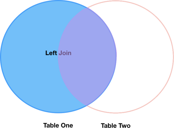
Left joins

What if we want to add information from buoys_df to wave_sub without losing any of the information from wave_sub? In this case, we use a different type of join called a “left outer join”, or a “left join”.

Like an inner join, a left join uses join keys to combine two DataFrames. Unlike an inner join, a left join will return all of the rows from the left DataFrame, even those rows whose join key(s) do not have values in the right DataFrame. Rows in the left DataFrame that are missing values for the join key(s) in the right DataFrame will simply have null (i.e., NaN or None) values for those columns in the resulting joined DataFrame.

Note: a left join will still discard rows from the right DataFrame that do not have values for the join key(s) in the left DataFrame.

A left join is performed in pandas by calling the same merge function used for inner join, but using the how='left' argument:

merged_left = pd.merge(left=wave_sub, right=buoys_df, how='left', left_on='buoy_id', right_on='buoy_id')
merged_left

The result DataFrame from a left join (merged_left) looks very much like the result DataFrame from an inner join (merged_inner) in terms of the columns it contains. However, unlike merged_inner, merged_left contains the same number of rows as the original wave_sub DataFrame. When we inspect merged_left, we find there are rows where the information that should have come from buoys_df (i.e. buoy_id, Name, Manufacturer, Depth, Type, operator, Country, Site, Type, latitude, and longitude). is missing (they contain NaN values):

merged_left[ pd.isnull(merged_left.Name_y) ]

These rows are the ones where the value of buoy_id from wave_sub (in this case, M6 Buoy) does not occur in buoys_df. Also note that where the two DataFrames have columns with the same name, Pandas appends _x to the column from the “left” dataframe, and _y to the column from the “right” dataframe.

Other join types

The pandas merge function supports two other join types:

• Right (outer) join: Invoked by passing how='right' as an argument. Similar to a left join, except all rows from the right DataFrame are kept, while rows from the left DataFrame without matching join key(s) values are discarded.
• Full (outer) join: Invoked by passing how='outer' as an argument. This join type returns the all pairwise combinations of rows from both DataFrames; i.e., the result DataFrame will NaN where data is missing in one of the dataframes. This join type is very rarely used.

Final Challenges

Challenge - Distributions

Create a new DataFrame by joining the contents of the waves.csv and buoys_data.csv tables. Then calculate the mean:

1. Wave Height by Site Type
2. Temperature by Seastate and by Country

Solution

# Merging the data frames
merged_left = pd.merge(left=waves_df,right=buoys_df, how='left', on="buoy_id")
# Group by Site Type, and calculate mean of Wave Height
merged_left.groupby("Type")["Wave Height"].mean()
# Group by Sea State and Country, and calculate mean of Temperature
merged_left.groupby(["Seastate","Country"])["Temperature"].mean()

Type
Directional                            3.489321
Downward-looking wave radar            0.600000
Unspecified wave measurement sensor    0.381098
Name: Wave Height, dtype: float64

Seastate  Country 
swell     England     17.324093
          Scotland    10.935880
          Wales       12.491667
windsea   England      9.300000
          Scotland     5.404502
          Wales       12.771239
Name: Temperature, dtype: float64

Challenge - filter by availability

1. In the data folder, there is a access.csv file that contains information about the data availability and access rights associated with each buoy. Use that data to summarize the number of observations which are reusable for research.
2. Again using access.csv file, use that data to summarize the number of data records from operational buoys which are available in Coastal versus Ocean waters.

Solution

1.

# Read the access file
access_df = pd.read_csv("data/access.csv")
# Merge the dataframes
merged_access = pd.merge(left=waves_df,right=access, how='left', on="buoy_id")
# find the number available for research
merged_access.groupby("data availability").count()
# or, this also gives the same answer:
merged_access[merged_access["data availability"]=="research"]

2.

buoy_access = pd.merge(left=buoys_df, right=access, how="left", on="buoy_id")
buoy_access[buoy_access["data availability"]=="operational"].groupby("Site Type")["buoy_id"].count()

Key Points

• Pandas’ merge and concat can be used to combine subsets of a DataFrame, or even data from different files.

• join function combines DataFrames based on index or column.

• Joining two DataFrames can be done in multiple ways (left, right, and inner) depending on what data must be in the final DataFrame.

• to_csv can be used to write out DataFrames in CSV format.