A brief introduction to geospatial data

Overview

Teaching: 30 min
Exercises: 45 min

Questions

• What can I do with geospatial data in Python?

• How can I visualise and analyse this data?

Objectives

• Import the Geopandas module to analyse latitude / longitude data.

• Use Geopandas and Geoplot to help with visualisation.

Geospatial Data

Often in the Environmental Sciences, we need to deal with geospatial data. This is normally presented as latitude and longitude (either as decimal degrees or as degrees/minutes/seconds), but can be presented in other formats (e.g. OSGB for UK Grid References).

A full discussion of geospatial vector data is beyond the scope of this episode - if you need more background please see this Carpentries Incubator lesson. Instead, we will highlight some useful tasks that can achieved with some key python libraries.

We’ll be using the data about buoys again.

import pandas as pd
buoys = pd.read_csv("data/buoy_data.csv",
                         keep_default_na=False, na_values=[""])

We can see that the dataset has a latitude and longitude. Let’s subset this data, along with the names.

locations = buoys[["Name", "latitude", "longitude"]]

To be able to deal with geospatial data, we need a python package that doesn’t come included with the Conda distribution we’re using. We can install the additional packages we need directly within a Notebook:

conda install geopandas -c conda-forge
conda install geoplot -c conda-forge

These might take several minutes to run. Once they’ve been installed, we can import them:

import geopandas as gpd
import geoplot as gplt

Conda environments

We’re now at the stage where you might find it useful to have different python environments for specific tasks. When you open Anaconda Navigator, it will, by default, be running in your base environment. However, you can create new environments via the Environments tab in the left-hand menu. Each environment can have different packages (or different versions of packages), different versions of python, etc - and different packages can be installed via the Environments tab. However, note that individual Notebooks are not associated with specific environments - they are associated with the current active environment. A full introduction to Conda environments can be found at https://carpentries-incubator.github.io/introduction-to-conda-for-data-scientists/

In our locations DataFrame, latitude and longitude are of type float:

locations.dtypes

Name          object
latitude     float64
longitude    float64
dtype: object

We need to convert the latitude and longitude to geometry data using Geopandas:

buoys_geo = gpd.GeoDataFrame(
    locations, geometry=gpd.points_from_xy(locations.longitude, locations.latitude), crs="EPSG:4326"
)

The value we’ve given to the crs argument specifies that the data is latitude and longitude, rather than any other coordinate system. We can now see that the buoys_geo DataFrame contains a new column, geometry, which also has type geometry.

So, what can we do with this data type?

Calculating distances

Calculating distances often involves some error if we need to convert between different coordinate types. Geopandas includes a distance function, but to calculate a distance in meters, we need to either project them in a local coordinate system to approximate the distance with a good precision, or use the Haversine equation (which is more accurate, but not implemented in Geopandas). In our case, we can project the data to the UK National Grid. The resulting distances will then be in metres:

buoys_geo.to_crs(epsg=27700,inplace=True)
buoys_geo["geometry"].distance(buoys_geo.iloc[0,3])

Notice the espg=27700 argument - this is the ESPG code for the UK National Grid. We have then calculated the distance of every point relative to the first point in the Series (Beryl A).

For the rest of the lesson, we need to consider the data back in Latitude / Longitude format, so let’s revert it back:

buoys_geo.to_crs(epsg="4326",inplace=True)

Geospatial polygons

In our case, the geospatial data are all individual points. However, geospatial data can also deal with polygons. Let’s load in data about Scottish Local Authority Boundaries:

scotland = gpd.read_file("data/scotland_boundaries.geojson")

We can immediately plot this:

scotland.plot()

We can see it looks like Scotland! We can look at the shape of the DataFrame to see that it has 32 rows - this is the number of Local Authorities in Scotland, and 5 columns.

We can find the “centroid” point of each Polygon - we can even plot this if we want an abstract map of Scotland!

scotland.centroid.plot()

We can also find the boundary length of each polygon. If we create add this to the DataFrame, then we can sort the resulting DataFrame and see which Council area has the shortest boundary:

scotland["lengths"] = scotland.length
scotland.sort_values("lengths")

Now, let’s look at a different geospatial file: the boundaries of the Cairngorms National Park, one of the National Parks in Scotland, and we can plot it

# Notice this is a different file format to the geojson file we used for the Scottish Council Boundaries data
# This is one file which makes up the Shapefile data format. At a minimum, there needs to be corresponding `shx` and `dbf` files (with the same filenames) in the same directory, but `prj`, `sbx`, `sbn`, and `shp.xml` can store additional metadata 
cairngorms =  gpd.read_file("data/cairngorms_boundary.shp")
cairngorms.plot()

Challenge: distances

This dataset also contains the length of the boundary, and the area of the National Park. Print these in km and square km, respectively

Solution

cairngorms.length/1000
cairngorms.area/1000000

One advantage of using geospatial data is seeing how things overlap. Geopandas contains an overlap method to find objects which have some (but not all) points in common. (There is also a similar intersects method.)

The overlap method can compare a single obect with a Series of objects, so let’s see which Scottish areas overlap with the Cairngorms National Park:

scotland.overlaps(cairngorms.iloc[0].geometry)

Challenge: overlaps

1. Subset the Scotland dataset to show only the rows which overlap with the Cairngorms. Can you display only the names?
2. Look in the Geopandas documentation (https://geopandas.org/en/stable/index.html) for the disjoint method. What do you think it will return when you run it in the way that we ran overlap? Try it - did you get the expected result? Can you plot this?

Solution

overlaps = scotland.overlaps(cairngorms.iloc[0].geometry)
# get a Series of only the overlaps
overlaps = overlaps.where(overlaps == True).dropna().index
OR, more concisely
overlaps = overlaps.index[overlaps]
# use this to subset the Scotland dataframe
scotland.loc[overlaps]
# ...and get the names
scotland.loc[overlaps].local_authority

disjoints = scotland.disjoint(cairngorms.iloc[0].geometry)
# get a Series of only the disjoints
disjoints = disjoints.index[disjoints]
# use this to subset the Scotland dataframe
disjoints = scotland.loc[disjoints]
disjoints.plot()

Challenge: plotting

We’ve already seen that we plot GeoDataFrames. We can pass these to Matplotlib subplots in the same way as any other figure. Can you plot the Scotland and Cairngorms GeoDataFrames on the same axes, and customise the plot to highlight the Cairngorms data in some way?

Solution

import matplotlib.pyplot as plt
figure, ax = plt.subplots()
scotland.plot(ax=ax)
cairngorms.plot(ax=ax, color="green")

Finally, Geopandas has a method to show geospatial data over an interactive map:

cairngorms.explore(style_kwds={"fillColor":"lime"})

We can even display the Cairngorms data directly over the Scotland plot, which validates that the result of our intersect command was correct

scotland_plot = scotland.explore()
cairngorms.explore(map=scotland_plot, style_kwds={"fillColor":"lime"})

Back to our buoy data

Our buoy data is based around the UK. Geopandas includes some very low resolution maps which we can use to plot our geospatial data on

world = gpd.read_file(gpd.datasets.get_path("naturalearth_lowres"))
ax = world.clip([-15, 50, 9, 61]).plot(color="white", edgecolor="black")
buoys_geo.plot(ax=ax, color="blue")

We use the clip() function to limit the bounds of the map to the most useful area for our needs.

What about if we want a higher quality map? There are several ways of achieving this. We’ve already seen that the explore() function gives us a way of generating an interactive map, but we can also use the Geoplot package, or Geopandas directly, to create maps. We’ll just use Geopandas, but Geoplot can give some more fine-grained control if you require it.

First, we need to import a basemap to plot buoy points onto.

north_atlantic = gpd.read_file("data/north_atlantic.geojson")

Where to find data

One challenge with mapping is often to find appropriate data. This file came from the NUTS dataset: https://marineregions.org/gazetteer.php?p=details&id=1912. Another useful source of European data is the EU (https://ec.europa.eu/eurostat/web/gisco/geodata/reference-data/administrative-units-statistical-units/nuts#nuts21), while the Cairngorms data we looked at earlier came from the UK Government geospatial data catalogue (https://www.data.gov.uk/dataset/8a00dbd7-e8f2-40e0-bcba-da2067d1e386/cairngorms-national-park-designated-boundary), and the Scottish data came from the Scottish Government (https://data.spatialhub.scot/dataset/local_authority_boundaries-is/resource/d24c5735-0f1c-4819-a6bd-dbfeb93bd8e4)

We can then plot the location of the buoys, and save the figure as we saw earlier. Although we could use the same technique as in the previous example (where we set the map as the axis and plotted the buoy positions on this object), here we’re showing we can also use Matplotlib subplots. This will allow us more control over the subsequent plot. However, subplots aren’t suppoorted directly via Pandas or Geopandas, so we now need to import Matplotlib

import matplotlib.pyplot as plt

fig, ax = plt.subplots()
north_atlantic.plot(ax=ax)
buoys_geo.plot(ax=ax, color="red")
plt.savefig("b.png")

Challenge - annotation

Earlier, we saw how to annotate figures. Can you annotate this map with the name of the buoy each dot represents?

Solution

import matplotlib.pyplot as plt

fig, ax = plt.subplots()
north_atlantic.plot(ax=ax)
buoys_geo.plot(ax=ax, color="red")

for buoy in buoys_geo.iterfeatures():
    ax.annotate(buoy["properties"]["Name"], xy=(buoy["properties"]["longitude"], buoy["properties"]["latitude"]))

The text is a little cramped! The next challenge will help fix this

Challenge

The North Atlantic dataset is comprised of lots of individual areas, which our buoys are all in 1 corner of. Can you:

• list the areas in the North Atlantic GeoDataFrame that include the buoy data
• set the bounds of the plot appropriately
• if you have time, investigate how you might customise the plot

Solution

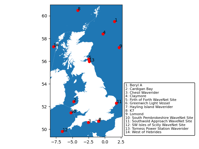
# the overlap function won't work, because it works on a 1-to-1 row-wise basis, whereas we 
want to find all the points which overlap with any of the areas
buoy_areas = north_atlantic.geometry.apply(lambda x: buoys_geo.within(x).any())
north_atlantic[buoy_areas]

# We can see that one of the areas is the "North Atlantic Ocean" - so this won't help fix the extent of the map!
# We can use a different way to set the bounds 

bounds = buoys_geo.total_bounds # The output of total_bounds is an array of minx,miny,maxx,maxy

fig, ax = plt.subplots()
ax.set_ylim([bounds[1]-0.5,bounds[3]+0.5])
ax.set_xlim([bounds[0]-0.5,bounds[2]+0.5])
north_atlantic.plot(ax=ax)

buoys_geo.plot(ax=ax, color="red")

for buoy in buoys_geo.iterfeatures():
    ax.annotate(buoy["properties"]["Name"], xy=(buoy["properties"]["longitude"], buoy["properties"]["latitude"]))

We could still improve the labels

# we additionally need this library for this example
from matplotlib.offsetbox import AnchoredText

bounds = buoys_geo.total_bounds

fig, ax = plt.subplots()
ax.set_ylim([bounds[1]-0.5,bounds[3]+0.5])
ax.set_xlim([bounds[0]-0.5,bounds[2]+0.5])
north_atlantic.plot(ax=ax)

buoys_geo.plot(ax=ax, color="red")

axis_labels = []

for buoy in buoys_geo.iterfeatures():
    ax.annotate(int(buoy["id"])+1, xy=(buoy["properties"]["longitude"], buoy["properties"]["latitude"]))
   axis_labels.append(f"{int(buoy['id'])+1}: {buoy['properties']['Name']}")

labels = AnchoredText("\n".join(axis_labels),
                       loc='lower left', prop=dict(size=8), frameon=True,
                       bbox_to_anchor=(1., 0),
                       bbox_transform=ax.transAxes
                       )
labels.patch.set_boxstyle("round,pad=0.,rounding_size=0.2")
ax.add_artist(labels) 
fig.tight_layout()

Hopefully this gives some insight into the power and control you have when using Matplotlib, and has given you some inspiration!

Key Points

• Geopandas is the key module to help deal with geospatial data.

• Using Geopandas and Geoplot we can create publication / web-ready maps.