Before we start
Overview
Teaching: 30 min
Exercises: 0 minQuestions
What is Python and why should I learn it?
Objectives
Present motivations for using Python.
Organize files and directories for a set of analyses as a Python project, and understand the purpose of the working directory.
How to work with Jupyter Notebook and Spyder.
Know where to find help.
Demonstrate how to provide sufficient information for troubleshooting with the Python user community.
What is Python?
Python is a general purpose programming language that supports rapid development of data analytics applications. The word “Python” is used to refer to both, the programming language and the tool that executes the scripts written in Python language.
Its main advantages are:
- Free
- Open-source
- Available on all major platforms (macOS, Linux, Windows)
- Supported by Python Software Foundation
- Supports multiple programming paradigms
- Has large community
- Rich ecosystem of third-party packages
So, why do you need Python for data analysis?
-
Easy to learn: Python is easier to learn than other programming languages. This is important because lower barriers mean it is easier for new members of the community to get up to speed.
-
Reproducibility: Reproducibility is the ability to obtain the same results using the same dataset(s) and analysis.
Data analysis written as a Python script can be reproduced on any platform. Moreover, if you collect more or correct existing data, you can quickly re-run your analysis!
An increasing number of journals and funding agencies expect analyses to be reproducible, so knowing Python will give you an edge with these requirements.
-
Versatility: Python is a versatile language that integrates with many existing applications to enable something completely amazing. For example, one can use Python to generate manuscripts, so that if you need to update your data, analysis procedure, or change something else, you can quickly regenerate all the figures and your manuscript will be updated automatically.
Python can read text files, connect to databases, and many other data formats, on your computer or on the web.
-
Interdisciplinary and extensible: Python provides a framework that allows anyone to combine approaches from different research (but not only) disciplines to best suit your analysis needs.
-
Python has a large and welcoming community: Thousands of people use Python daily. Many of them are willing to help you through mailing lists and websites, such as Stack Overflow and Anaconda community portal.
-
Free and Open-Source Software (FOSS)… and Cross-Platform: We know we have already said that but it is worth repeating.
Knowing your way around Anaconda
Anaconda distribution of Python includes a lot of its popular packages, such as the IPython console, Jupyter Notebook, and Spyder IDE. Have a quick look around the Anaconda Navigator. You can launch programs from the Navigator or use the command line.
The Jupyter Notebook is an open-source web application that allows you to create and share documents that allow one to create documents that combine code, graphs, and narrative text. Spyder is an Integrated Development Environment that allows one to write Python scripts and interact with the Python software from within a single interface.
Anaconda also comes with a package manager called conda, which makes it easy to install and update additional packages.
Research Project: Best Practices
It is a good idea to keep a set of related data, analyses, and text in a single folder. All scripts and text files within this folder can then use relative paths to the data files. Working this way makes it a lot easier to move around your project and share it with others.
Organizing your working directory
Using a consistent folder structure across your projects will help you keep things organized, and will also make it easy to find/file things in the future. This can be especially helpful when you have multiple projects. In general, you may wish to create separate directories for your scripts, data, and documents.
-
data/: Use this folder to store your raw data. For the sake of transparency and provenance, you should always keep a copy of your raw data. If you need to cleanup data, do it programmatically (i.e. with scripts) and make sure to separate cleaned up data from the raw data. For example, you can store raw data in files./data/raw/and clean data in./data/clean/. -
documents/: Use this folder to store outlines, drafts, and other text. -
code/: Use this folder to store your (Python) scripts for data cleaning, analysis, and plotting that you use in this particular project.
You may need to create additional directories depending on your project needs, but these should form
the backbone of your project’s directory. For this workshop, we will need a data/ folder to store
our raw data, and we will later create a data_output/ folder when we learn how to export data as
CSV files.
What is Programming and Coding?
Programming is the process of writing “programs” that a computer can execute and produce some (useful) output. Programming is a multi-step process that involves the following steps:
- Identifying the aspects of the real-world problem that can be solved computationally
- Identifying (the best) computational solution
- Implementing the solution in a specific computer language
- Testing, validating, and adjusting implemented solution.
While “Programming” refers to all of the above steps, “Coding” refers to step 3 only: “Implementing the solution in a specific computer language”. It’s important to note that “the best” computational solution must consider factors beyond the computer. Who is using the program, what resources/funds does your team have for this project, and the available timeline all shape and mold what “best” may be.
If you are working with Jupyter notebook:
You can type Python code into a code cell and then execute the code by pressing
Shift+Return.
Output will be printed directly under the input cell.
You can recognise a code cell by the In[ ]: at the beginning of the cell and output by Out[ ]:.
Pressing the + button in the menu bar will add a new cell.
All your commands as well as any output will be saved with the notebook.
If you are working with Spyder:
You can either use the console or use script files (plain text files that contain your code). The console pane (in Spyder, the bottom right panel) is the place where commands written in the Python language can be typed and executed immediately by the computer. It is also where the results will be shown. You can execute commands directly in the console by pressing Return, but they will be “lost” when you close the session. Spyder uses the IPython console by default.
Since we want our code and workflow to be reproducible, it is better to type the commands in the script editor, and save them as a script. This way, there is a complete record of what we did, and anyone (including our future selves!) has an easier time reproducing the results on their computer.
Spyder allows you to execute commands directly from the script editor by using the run buttons on top. To run the entire script click Run file or press F5, to run the current line click Run selection or current line or press F9, other run buttons allow to run script cells or go into debug mode. When using F9, the command on the current line in the script (indicated by the cursor) or all of the commands in the currently selected text will be sent to the console and executed.
At some point in your analysis you may want to check the content of a variable or the structure of an object, without necessarily keeping a record of it in your script. You can type these commands and execute them directly in the console. Spyder provides the Ctrl+Shift+E and Ctrl+Shift+I shortcuts to allow you to jump between the script and the console panes.
If Python is ready to accept commands, the IPython console shows an In [..]: prompt with the
current console line number in []. If it receives a command (by typing, copy-pasting or sent from
the script editor), Python will execute it, display the results in the Out [..]: cell, and come
back with a new In [..]: prompt waiting for new commands.
If Python is still waiting for you to enter more data because it isn’t complete yet, the console
will show a ...: prompt. It means that you haven’t finished entering a complete command. This can
be because you have not typed a closing parenthesis (), ], or }) or quotation mark. When this
happens, and you thought you finished typing your command, click inside the console window and press
Esc; this will cancel the incomplete command and return you to the In [..]: prompt.
How to learn more after the workshop?
The material we cover during this workshop will give you an initial taste of how you can use Python to analyze data for your own research. However, you will need to learn more to do advanced operations such as cleaning your dataset, using statistical methods, or creating beautiful graphics. The best way to become proficient and efficient at python, as with any other tool, is to use it to address your actual research questions. As a beginner, it can feel daunting to have to write a script from scratch, and given that many people make their code available online, modifying existing code to suit your purpose might make it easier for you to get started.
Seeking help
- check under the Help menu
- type
help() - type
?objectorhelp(object)to get information about an object - Python documentation
- Pandas documentation
Finally, a generic Google or internet search “Python task” will often either send you to the appropriate module documentation or a helpful forum where someone else has already asked your question.
I am stuck… I get an error message that I don’t understand. Start by googling the error message. However, this doesn’t always work very well, because often, package developers rely on the error catching provided by Python. You end up with general error messages that might not be very helpful to diagnose a problem (e.g. “subscript out of bounds”). If the message is very generic, you might also include the name of the function or package you’re using in your query.
However, you should check Stack Overflow. Search using the [python] tag. Most questions have already
been answered, but the challenge is to use the right words in the search to find the answers:
https://stackoverflow.com/questions/tagged/python?tab=Votes
Asking for help
The key to receiving help from someone is for them to rapidly grasp your problem. You should make it as easy as possible to pinpoint where the issue might be.
Try to use the correct words to describe your problem. For instance, a package is not the same thing as a library. Most people will understand what you meant, but others have really strong feelings about the difference in meaning. The key point is that it can make things confusing for people trying to help you. Be as precise as possible when describing your problem.
If possible, try to reduce what doesn’t work to a simple reproducible example. If you can reproduce the problem using a very small data frame instead of your 50,000 rows and 10,000 columns one, provide the small one with the description of your problem. When appropriate, try to generalize what you are doing so even people who are not in your field can understand the question. For instance, instead of using a subset of your real dataset, create a small (3 columns, 5 rows) generic one.
Where to ask for help?
- The person sitting next to you during the workshop. Don’t hesitate to talk to your neighbor during the workshop, compare your answers, and ask for help. You might also be interested in organizing regular meetings following the workshop to keep learning from each other.
- Your friendly colleagues: if you know someone with more experience than you, they might be able and willing to help you.
- Stack Overflow: if your question hasn’t been answered before and is well crafted, chances are you will get an answer in less than 5 min. Remember to follow their guidelines on how to ask a good question.
- Python mailing lists
More resources
Key Points
Python is an open source and platform independent programming language.
Jupyter Notebook and the Spyder IDE are great tools to code in and interact with Python. With the large Python community it is easy to find help on the internet.
Short Introduction to Programming in Python
Overview
Teaching: 30 min
Exercises: 5 minQuestions
How do I program in Python?
How can I represent my data in Python?
Objectives
Describe the advantages of using programming vs. completing repetitive tasks by hand.
Define the following data types in Python: strings, integers, and floats.
Perform mathematical operations in Python using basic operators.
Define the following as it relates to Python: lists, tuples, and dictionaries.
Refresher (hopefully!)
Hopefully, everything on this page should be familiar to everyone on this course! There’s a chance some of the attendees may not have have done the functions episode
Interpreter
Python is an interpreted language which can be used in two ways:
- “Interactively”: when you use it as an “advanced calculator” executing
one command at a time. To start Python in this mode, execute
pythonon the command line:
$ python
Python 3.5.1 (default, Oct 23 2015, 18:05:06)
[GCC 4.8.3] on linux2
Type "help", "copyright", "credits" or "license" for more information.
>>>
Chevrons >>> indicate an interactive prompt in Python, meaning that it is waiting for your
input.
2 + 2
4
print("Hello World")
Hello World
- “Scripting” Mode: executing a series of “commands” saved in text file,
usually with a
.pyextension after the name of your file:
$ python my_script.py
Hello World
Introduction to variables in Python
Assigning values to variables
One of the most basic things we can do in Python is assign values to variables:
text = "Data Carpentry"  # An example of assigning a value to a new text variable,
                         # also known as a string data type in Python
number = 42              # An example of assigning a numeric value, or an integer data type
pi_value = 3.1415        # An example of assigning a floating point value (the float data type)
Here we’ve assigned data to the variables text, number and pi_value,
using the assignment operator =. To review the value of a variable, we
can type the name of the variable into the interpreter and press Return:
text
"Data Carpentry"
Everything in Python has a type. To get the type of something, we can pass it
to the built-in function type:
type(text)
<class 'str'>
type(number)
<class 'int'>
type(pi_value)
<class 'float'>
The variable text is of type str, short for “string”. Strings hold
sequences of characters, which can be letters, numbers, punctuation
or more exotic forms of text (even emoji!).
We can also see the value of something using another built-in function, print:
print(text)
Data Carpentry
print(number)
42
This may seem redundant, but in fact it’s the only way to display output in a script:
example.py
# A Python script file
# Comments in Python start with #
# The next line assigns the string "Data Carpentry" to the variable "text".
text = "Data Carpentry"

# The next line does nothing!
text

# The next line uses the print function to print out the value we assigned to "text"
print(text)
Running the script
$ python example.py
Data Carpentry
Notice that “Data Carpentry” is printed only once.
Tip: print and type are built-in functions in Python. Later in this
lesson, we will introduce methods and user-defined functions. The Python
documentation is excellent for reference on the differences between them.
Operators
We can perform mathematical calculations in Python using the basic operators
+, -, /, *, %:
2 + 2 # Addition
4
6 * 7 # Multiplication
42
2 ** 16 # Power
65536
13 % 5 # Modulo
3
We can also use comparison and logic operators:
<, >, ==, !=, <=, >= and statements of identity such as
and, or, not. The data type returned by this is
called a boolean.
3 > 4
False
True and True
True
True or False
True
True and False
False
Sequences: Lists and Tuples
Lists
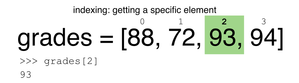
Lists are a common data structure to hold an ordered sequence of elements. Each element can be accessed by an index. Note that Python indexes start with 0 instead of 1:
numbers = [1, 2, 3]
numbers[0]
1
A for loop can be used to access the elements in a list or other Python data
structure one at a time:
for num in numbers:
    print(num)
1
2
3
Indentation is very important in Python. Note that the second line in the
example above is indented. Just like three chevrons >>> indicate an
interactive prompt in Python, the three dots ... are Python’s prompt for
multiple lines. This is Python’s way of marking a block of code. [Note: you
do not type >>> or ....]
To add elements to the end of a list, we can use the append method. Methods
are a way to interact with an object (a list, for example). We can invoke a
method using the dot . followed by the method name and a list of arguments
in parentheses. Let’s look at an example using append:
numbers.append(4)
print(numbers)
[1, 2, 3, 4]
To find out what methods are available for an
object, we can use the built-in help command:
help(numbers)

Help on list object:

class list(object)
 |  list() -> new empty list
 |  list(iterable) -> new list initialized from iterable's items
 ...
Tuples
A tuple is similar to a list in that it’s an ordered sequence of elements.
However, tuples can not be changed once created (they are “immutable”). Tuples
are created by placing comma-separated values inside parentheses ().
# Tuples use parentheses
a_tuple = (1, 2, 3)
another_tuple = ('blue', 'green', 'red')

# Note: lists use square brackets
a_list = [1, 2, 3]
Tuples vs. Lists
- What happens when you execute
a_list[1] = 5?- What happens when you execute
a_tuple[2] = 5?- What does
type(a_tuple)tell you abouta_tuple?- What information does the built-in function
len()provide? Does it provide the same information on both tuples and lists? Does thehelp()function confirm this?Solution
1. The second value in a_list is replaced with 5.
2. There is an error:
TypeError: 'tuple' object does not support item assignmentAs a tuple is immutable, it does not support item assignment. Elements in a list can be altered individually.
3.
<class 'tuple'>; The function tells you that the variablea_tupleis an object of the class tuple.4.
len()tells us the length of an object. It works the same for both lists and tuples, providing us with the number of entries in each case.
Dictionaries
A dictionary is a container that holds pairs of objects - keys and values.
translation = {'one': 'first', 'two': 'second'}
translation['one']
'first'
Dictionaries work a lot like lists - except that you index them with keys. You can think about a key as a name or unique identifier for the value it corresponds to.
rev = {'first': 'one', 'second': 'two'}
rev['first']
'one'
To add an item to the dictionary we assign a value to a new key:
rev['third'] = 'three'
rev
{'first': 'one', 'second': 'two', 'third': 'three'}
Using for loops with dictionaries is a little more complicated. We can do
this in two ways:
for key, value in rev.items():
    print(key, '->', value)
'first' -> one
'second' -> two
'third' -> three
or
for key in rev.keys():
    print(key, '->', rev[key])
'first' -> one
'second' -> two
'third' -> three
Changing dictionaries
- First, print the value of the
revdictionary to the screen.- Reassign the value that corresponds to the key
secondso that it no longer reads “two” but instead2.- Print the value of
revto the screen again to see if the value has changed.Solution
1.
print(rev){'first': 'one', 'second': 'two', 'third': 'three'}2 & 3:
rev['second'] = 2
print(rev)
{'first': 'one', 'second': 2, 'third': 'three'}
Functions
Defining a section of code as a function in Python is done using the def
keyword. For example a function that takes two arguments and returns their sum
can be defined as:
def add_function(a, b):
    result = a + b
    return result

z = add_function(20, 22)
print(z)
42
Key Points
Python is an interpreted language which can be used interactively (executing one command at a time) or in scripting mode (executing a series of commands saved in file).
One can assign a value to a variable in Python. Those variables can be of several types, such as string, integer, floating point and complex numbers.
Lists and tuples are similar in that they are ordered lists of elements; they differ in that a tuple is immutable (cannot be changed).
Dictionaries are data structures that provide mappings between keys and values.
Starting With Data
Overview
Teaching: 30 min
Exercises: 30 minQuestions
How can I import data in Python?
What is Pandas?
Why should I use Pandas to work with data?
Objectives
Navigate the workshop directory and download a dataset.
Explain what a library is and what libraries are used for.
Describe what the Python Data Analysis Library (Pandas) is.
Load the Python Data Analysis Library (Pandas).
Read tabular data into Python using Pandas.
Describe what a DataFrame is in Python.
Access and summarize data stored in a DataFrame.
Define indexing as it relates to data structures.
Perform basic mathematical operations and summary statistics on data in a Pandas DataFrame.
Create simple plots.
Working With Pandas DataFrames in Python
We can automate the process of performing data manipulations in Python. It’s efficient to spend time building the code to perform these tasks because once it’s built, we can use it over and over on different datasets that use a similar format. This makes our methods easily reproducible. We can also easily share our code with colleagues and they can replicate the same analysis.
Starting in the same spot
To help the lesson run smoothly, let’s ensure everyone is in the same directory. This should help us avoid path and file name issues. At this time please navigate to the workshop directory. If you are working in Jupyter Notebook be sure that you start your notebook in the workshop directory.
A quick aside that there are Python libraries like OS Library that can work with our directory structure, however, that is not our focus today.
Our Data
We are studying ocean waves and temperature in the seas around the UK.
For this lesson we will be using a subset of data from Centre for Environment Fisheries and Aquaculture Science (Cefas). WaveNet, Cefas’ strategic wave monitoring network for the United Kingdom, provides a single source of real-time wave data from a network of wave buoys located in areas at risk from flooding. https://wavenet.cefas.co.uk/
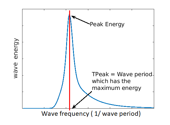
If we look out to sea, we notice that waves on the sea surface are not simple sinusoids. The surface appears to be composed of random waves of various lengths and periods. How can we describe this complex surface?
By making some simplifications and assumptions, we fit an idealised ‘spectrum’ to describe all the energy held in different wave frequencies. This describes the wave energy at a point, covering the energy in small ripples (high frequency) to long period (low frequency) swell waves. This figure shows an example idealised spectrum, with the highest energy around wave periods of 11 seconds.
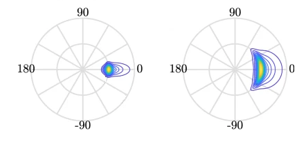
We can go a step further, and also associate a wave direction with the amount of energy. These simplifications lead to a 2D wave spectrum at any point in the sea, with dimensions frequency and direction. Directional spreading is a measure of how wave energy for a given sea state is spread as a function of direction of propagation. For example the wave data on the left have a small directional spread, as the waves travel, this can fan out over a wider range of directions.
When it is very windy or storms pass-over large sea areas, surface waves grow from short choppy wind-sea waves into powerful swell waves. The height and energy of the waves is larger in winter time, when there are more storms. wind-sea waves have short wavelengths / wave periods (like ripples) while swell waves have longer periods (at a lower frequency).
The example file contains a obervations of sea temperatures, and waves properties at different buoys around the UK.
The dataset is stored as a .csv file: each row holds information for a
single wave buoy, and the columns represent:
| Column | Description |
|---|---|
| record_id | Unique id for the observation |
| buoy_id | Unique id for the wave buoy |
| Name | Name of the wave buoy |
| Date | Date & time of measurement in day/month/year hour:minute |
| Tz | The average wave period (in seconds) |
| Peak Direction | The direction of the highest energy waves (in degrees) |
| Tpeak | The period of the highest energy waves (in seconds) |
| Wave Height | Significant* wave height (in metres) |
| Temperature | Water temperature (in degrees C) |
| Spread | The “directional spread” at Tpeak (in degrees) |
| Operations | Sea safety classification |
| Seastate | Categorised by period |
| Quadrant | Categorised by prevailing wave direction |
* “significant” here is defined as the mean wave height (trough to crest) of the highest third of the waves
The first few rows of our first file look like this:
record_id,buoy_id,Name,Date,Tz,Peak Direction,Tpeak,Wave,Height,Temperature,Spread,Operations,Seastate,Quadrant
1,14,SW Isles of Scilly WaveNet Site,17/04/2023,00:00,7.2,263,10,1.8,10.8,26,crew,swell,west
2,7,Hayling Island Waverider,17/04/2023,00:00,4,193,11.1,0.2,10.2,14,crew,swell,south
3,5,Firth of Forth WaveNet Site,17/04/2023,00:00,3.7,115,4.5,0.6,7.8,28,crew,windsea,east
4,3,Chesil Waverider,17/04/2023,00:00,5.5,225,8.3,0.5,10.2,48,crew,swell,south
5,10,M6 Buoy,17/04/2023,00:00,7.6,240,11.7,4.5,11.5,89,no,go,swell,west
6,9,Lomond,17/04/2023,00:00,4,NaN,NaN,0.5,NaN,NaN,crew,swell,north
About Libraries
A library in Python contains a set of tools (called functions) that perform tasks on our data. Importing a library is like getting a piece of lab equipment out of a storage locker and setting it up on the bench for use in a project. Once a library is set up, it can be used or called to perform the task(s) it was built to do.
Pandas in Python
One of the best options for working with tabular data in Python is to use the Python Data Analysis Library (a.k.a. Pandas). The Pandas library provides data structures, produces high quality plots with matplotlib and integrates nicely with other libraries that use NumPy (which is another Python library) arrays.
Python doesn’t load all of the libraries available to it by default. We have to
add an import statement to our code in order to use library functions. To import
a library, we use the syntax import libraryName. If we want to give the
library a nickname to shorten the command, we can add as nickNameHere. An
example of importing the pandas library using the common nickname pd is below.
import pandas as pd
Each time we call a function that’s in a library, we use the syntax
LibraryName.FunctionName. Adding the library name with a . before the
function name tells Python where to find the function. In the example above, we
have imported Pandas as pd. This means we don’t have to type out pandas each
time we call a Pandas function.
Reading CSV Data Using Pandas
We will begin by locating and reading our wave data which are in CSV format. CSV stands for
Comma-Separated Values and is a common way to store formatted data. Other symbols may also be used, so
you might see tab-separated, colon-separated or space separated files. It is quite easy to replace
one separator with another, to match your application. The first line in the file often has headers
to explain what is in each column. CSV (and other separators) make it easy to share data, and can be
imported and exported from many applications, including Microsoft Excel. For more details on CSV
files, see the Data Organisation in Spreadsheets lesson.
We can use Pandas’ read_csv function to pull the file directly into a DataFrame.
So What’s a DataFrame?
A DataFrame is a 2-dimensional data structure that can store data of different
types (including characters, integers, floating point values, factors and more)
in columns. It is similar to a spreadsheet or an SQL table or the data.frame in
R. A DataFrame always has an index (0-based). An index refers to the position of
an element in the data structure.
# Note that pd.read_csv is used because we imported pandas as pd
pd.read_csv("data/waves.csv")
Referring to libraries
If you import a library using its full name, you need to use that name when using functions from it. If you use a nickname, you can only use the nickname when calling functions from that library For example, if you use
import pandas, you would need to writepandas.read_csv(...), but if you useimport pandas as pd, writingpandas.read_csv(...)will show an error ofname 'pandas' is not defined
The above command yields the output below:
,record_id,buoy_id,Name,Date,Tz,Peak Direction,Tpeak,Wave Height,Temperature,Spread,Operations,Seastate,Quadrant
0,1,14,SW Isles of Scilly WaveNet Site,17/04/2023 00:00,7.2,263.0,10.0,1.80,10.80,26.0,crew,swell,west
1,2,7,Hayling Island Waverider,17/04/2023 00:00,4.0,193.0,11.1,0.20,10.20,14.0,crew,swell,south
2,3,5,Firth of Forth WaveNet Site,17/04/2023 00:00,3.7,115.0,4.5,0.60,7.80,28.0,crew,windsea,east
3,4,3,Chesil Waverider,17/04/2023 00:00,5.5,225.0,8.3,0.50,10.20,48.0,crew,swell,south
4,5,10,M6 Buoy,17/04/2023 00:00,7.6,240.0,11.7,4.50,11.50,89.0,no go,swell,west
...,...,...,...,...,...,...,...,...,...,...,...,...,...
2068,2069,16,west of Hebrides,18/10/2022 16:00,6.1,13.0,9.1,1.46,12.70,28.0,crew,swell,north
2069,2070,16,west of Hebrides,18/10/2022 16:30,5.9,11.0,8.7,1.49,12.70,34.0,crew,swell,north
2070,2071,16,west of Hebrides,18/10/2022 17:00,5.6,3.0,9.5,1.36,12.65,34.0,crew,swell,north
2071,2072,16,west of Hebrides,18/10/2022 17:30,5.7,347.0,10.0,1.39,12.70,31.0,crew,swell,north
2072,2073,16,west of Hebrides,18/10/2022 18:00,5.7,8.0,8.7,1.36,12.65,34.0,crew,swell,north
2073 rows × 13 columns
We can see that there were 2073 rows parsed. Each row has 13
columns. The first column is the index of the DataFrame. The index is used to
identify the position of the data, but it is not an actual column of the DataFrame
(but note that in this instance we also have a record_id which is the same as the index, and
is a column of the DataFrame).
It looks like the read_csv function in Pandas read our file properly. However,
we haven’t saved any data to memory so we can work with it. We need to assign the
DataFrame to a variable. Remember that a variable is a name for a value, such as x,
or data. We can create a new object with a variable name by assigning a value to it using =.
Let’s call the imported wave data waves_df:
waves_df = pd.read_csv("data/waves.csv")
Notice when you assign the imported DataFrame to a variable, Python does not
produce any output on the screen. We can view the value of the waves_df
object by typing its name into the Python command prompt.
waves_df
which prints contents like above.
Note: if the output is too wide to print on your narrow terminal window, you may see something slightly different as the large set of data scrolls past. You may see simply the last column of data. Never fear, all the data is there, if you scroll up.
If we selecting just a few rows, so it is easier to fit on one window, you can see that pandas has neatly formatted the data to fit our screen:
waves_df.head() # The head() method displays the first several lines of a file. It is discussed below.
,record_id,buoy_id,Name,Date,Tz,Peak Direction,Tpeak,Wave Height,Temperature,Spread,Operations,Seastate,Quadrant
0,1,14,SW Isles of Scilly WaveNet Site,17/04/2023 00:00,7.2,263.0,10.0,1.80,10.80,26.0,crew,swell,west
1,2,7,Hayling Island Waverider,17/04/2023 00:00,4.0,193.0,11.1,0.20,10.20,14.0,crew,swell,south
2,3,5,Firth of Forth WaveNet Site,17/04/2023 00:00,3.7,115.0,4.5,0.60,7.80,28.0,crew,windsea,east
3,4,3,Chesil Waverider,17/04/2023 00:00,5.5,225.0,8.3,0.50,10.20,48.0,crew,swell,south
4,5,10,M6 Buoy,17/04/2023 00:00,7.6,240.0,11.7,4.50,11.50,89.0,no go,swell,west
Exploring Our Wave Buoy Data
Again, we can use the type function to see what kind of thing waves_df is:
type(waves_df)
<class 'pandas.core.frame.DataFrame'>
As expected, it’s a DataFrame (or, to use the full name that Python uses to refer
to it internally, a pandas.core.frame.DataFrame).
What kind of things does waves_df contain? DataFrames have an attribute
called dtypes that answers this:
waves_df.dtypes
record_id           int64
buoy_id             int64
Name               object
Date               object
Tz                float64
Peak Direction    float64
Tpeak             float64
Wave Height       float64
Temperature       float64
Spread            float64
Operations         object
Seastate           object
Quadrant           object
dtype: object
All the values in a column have the same type. For example, buoy_id have type
int64, which is a kind of integer. Cells in the buoy_id column cannot have
fractional values, but the TPeak and Wave Height columns can, because they
have type float64. The object type doesn’t have a very helpful name, but in
this case it represents strings (such as ‘swell’ and ‘windsea’ in the case of Seastate).
We’ll talk a bit more about what the different formats mean in a different lesson.
Useful Ways to View DataFrame Objects in Python
There are many ways to summarize and access the data stored in DataFrames, using attributes and methods provided by the DataFrame object.
To access an attribute, use the DataFrame object name followed by the attribute
name df_object.attribute. Using the DataFrame waves_df and attribute
columns, an index of all the column names in the DataFrame can be accessed
with waves_df.columns.
Methods are called in a similar fashion using the syntax df_object.method().
As an example, waves_df.head() gets the first few rows in the DataFrame
waves_df using the head() method. With a method we can supply extra
information in the parens to control behaviour.
Let’s look at the data using these.
Challenge - DataFrames
Using our DataFrame
waves_df, try out the attributes & methods below to see what they return.
waves_df.columnswaves_df.shapeTake note of the output ofshape- what format does it return the shape of the DataFrame in? HINT: More on tuples herewaves_df.head()Also, what doeswaves_df.head(15)do?waves_df.tail()Solution
Index(['record_id', 'buoy_id', 'Name', 'Date', 'Tz', 'Peak Direction', 'Tpeak',
   'Wave Height', 'Temperature', 'Spread', 'Operations', 'Seastate',
   'Quadrant'],
   dtype='object')
2.
(2073, 13)It is a tuple
3.
  record_id  buoy_id  ... Seastate Quadrant
0          1       14  ...    swell     west
1          2        7  ...    swell    south
2          3        5  ...  windsea     east
3          4        3  ...    swell    south
4          5       10  ...    swell     west
[5 rows x 13 columns]
So,
waves_df.head()returns the first 5 rows of thewaves_dfdataframe. (Your Jupyter Notebook might show all columns).waves_df.head(15)returns the first 15 rows; i.e. the default value (recall the functions lesson) is 5, but we can change this via an argument to the function4.
      record_id  buoy_id              Name  ... Operations  Seastate  Quadrant
2068       2069       16  west of Hebrides  ...       crew     swell     north
2069       2070       16  west of Hebrides  ...       crew     swell     north
2070       2071       16  west of Hebrides  ...       crew     swell     north
2071       2072       16  west of Hebrides  ...       crew     swell     north
2072       2073       16  west of Hebrides  ...       crew     swell     north

[5 rows x 13 columns]
So,
waves_df.tail()returns the final 5 rows of the dataframe. We can also control the output by adding an argument, like withhead()
Calculating Statistics From Data In A Pandas DataFrame
We’ve read our data into Python. Next, let’s perform some quick summary statistics to learn more about the data that we’re working with. We might want to know how many observations were collected in each site, or how many observations were made at each named buoy. We can perform summary stats quickly using groups. But first we need to figure out what we want to group by.
Let’s begin by exploring our data:
# Look at the column names
waves_df.columns
which returns:
Index(['record_id', 'buoy_id', 'Name', 'Date', 'Tz', 'Peak Direction', 'Tpeak',
       'Wave Height', 'Temperature', 'Spread', 'Operations', 'Seastate',
       'Quadrant'],
      dtype='object')
Let’s get a list of all the buoys. The pd.unique function tells us all of
the unique values in the Name column.
pd.unique(waves_df['Name'])
which returns:
array(['SW Isles of Scilly WaveNet Site', 'Hayling Island Waverider',
       'Firth of Forth WaveNet Site', 'Chesil Waverider', 'M6 Buoy',
       'Lomond', 'Cardigan Bay', 'South Pembrokeshire WaveNet Site',
       'Greenwich Light Vessel', 'west of Hebrides'], dtype=object)
Challenge - Statistics
Create a list of unique site IDs (“buoy_id”) found in the waves data. Call it
buoy_ids. How many unique buoys are in the data?What is the difference between using
len(buoy_ids)andwaves_df['buoy_id'].nunique()? in this case, the result is the same but when might be the difference be important?Solution
1.
buoy_ids = pd.unique(waves_df["buoy_id"])
print(buoy_ids)
[14 7 5 3 10 9 2 11 6 16]2.
We could count the number of elements of the list, or we might think about using either the
len()ornunique()functions, and we get 10.We can see the difference between
len()andnunique()if we create a DataFrame with aNonevalue:length_test = pd.DataFrame([1,2,3,None]) print(len(length_test)) print(length_test.nunique())We can see that
len()returns 4, whilenunique()returns 3 - this is becausenunique()ignore anyNullvalue
Groups in Pandas
We often want to calculate summary statistics grouped by subsets or attributes within fields of our data. For example, we might want to calculate the average Wave Height at all buoys per Seastate.
We can calculate basic statistics for all records in a single column using the syntax below:
waves_df['Temperature'].describe()
which gives the following
count    1197.000000
mean       12.872891
std         4.678751
min         5.150000
25%        12.200000
50%        12.950000
75%        17.300000
max        18.700000
Name: Temperature, dtype: float64
What counts don’t include
Note that the value of
countis not the same as the total number of rows. This is because statistical methods in Pandas ignore NaN (“not a number”) values. We can count the total number of of NaNs usingwaves_df["Temperature"].isna().sum(), which returns 876. 876 + 1197 is 2073, which is the total number of rows in the DataFrame
We can also extract one specific metric if we wish:
waves_df['Temperature'].min()
waves_df['Temperature'].max()
waves_df['Temperature'].mean()
waves_df['Temperature'].std()
waves_df['Temperature'].count()
But if we want to summarize by one or more variables, for example Seastate, we can
use Pandas’ .groupby method. Once we’ve created a groupby DataFrame, we
can quickly calculate summary statistics by a group of our choice.
# Group data by Seastate
grouped_data = waves_df.groupby('Seastate')
The Pandas describe function will return descriptive stats including: mean,
median, max, min, std and count for a particular column in the data. Pandas’
describe function will only return summary values for columns containing
numeric data (does this always make sense?)
# Summary statistics for all numeric columns by Seastate
grouped_data.describe()
# Provide the mean for each numeric column by Seastate
grouped_data.mean(numeric_only=True)
grouped_data.mean(numeric_only=True) produces
record_id,buoy_id,...,Temperature,Spread
,count,mean,std,min,25%,50%,75%,max,count,mean,...,75%,max,count,mean,std,min,25%,50%,75%,max
Seastate,
swell,1747.0,1019.925587,645.553036,1.0,441.50,878.0,1636.5,2073.0,1747.0,11.464797,...,17.4000,18.70,378.0,30.592593,10.035383,14.0,23.0,28.0,36.0,89.0
windsea,326.0,1128.500000,188.099299,3.0,1036.25,1121.5,1273.5,1355.0,326.0,7.079755,...,12.4875,13.35,326.0,25.036810,9.598327,9.0,16.0,25.0,31.0,68.0
2 rows × 64 columns
The groupby command is powerful in that it allows us to quickly generate
summary stats.
This example shows that the wave height associated with water described as ‘swell’ is much larger than the wave heights classified as ‘windsea’.
Challenge - Summary Data
- How many records have the prevailing wave direction (Quadrant) ‘north’ and how many ‘west’?
- What happens when you group by two columns using the following syntax and then calculate mean values?
grouped_data2 = waves_df.groupby(['Seastate', 'Quadrant'])grouped_data2.mean()- Summarize Temperature values for swell and windsea states in your data.
Solution
- The most complete answer is
waves_df.groupby("Quadrant").count()["record_id"][["north", "west"]]- note that we could use any column that has a value in every row - but given thatrecord_idis our index for the dataset it makes sense to use that- It groups by 2nd column within the results of the 1st column, and then calculates the mean (n.b. depending on your version of python, you might need
grouped_data2.mean(numeric_only=True))waves_df.groupby(['Seastate'])["Temperature"].describe()which produces the following:
            count    mean         std         min     25%      50%      75%        max
Seastate
   swell    871.0    14.703502    3.626322    5.15    12.75    17.10    17.4000    18.70
 windsea    326.0    7.981902     3.518419    5.15     5.40     5.45    12.4875    13.35
Quickly Creating Summary Counts in Pandas
Let’s next count the number of records for each buoy. We can do this in a few
ways, but we’ll use groupby combined with a count() method.
# Count the number of samples by Name
name_counts = waves_df.groupby('Name')['record_id'].count()
print(name_counts)
Or, we can also count just the rows that have the Name “SW Isle of Scilly WaveNet Site”:
waves_df.groupby('Name')['record_id'].count()['SW Isles of Scilly WaveNet Site']
Basic Maths Functions
If we wanted to, we could perform math on an entire column of our data. For example let’s convert all the degrees values to radians.
# convert the directions from degrees to radians
# Sometimes people use different units for directions, for example we could describe
# the directions in terms of radians (where a full circle 360 degrees = 2*pi radians)
# To do this we need to use the math library which contains the constant pi

# Convert degrees to radians by multiplying all direction values values by pi/180
import math # the constant pi is stored in the math(s) library, so need to import it
waves_df['Peak Direction'] * math.pi / 180
Constants
It is normal for code to include variables that have values that should not change, for example. the mathematical value of pi. These are called constants. The maths library contains three numerical constants: pi, e, and tau, but other built-in modules also contain constants. The
oslibrary (which provides a portable way of using operating system tools, such as creating directories) lists error codes as constants, while thecalendarlibrary contains the days of the week mapped to numerical index (from monday as zero) as constants.The convention for naming constants is to use block capitals (n.b.
math.pidoesn’t follow this!) and to list them all together at the top of a module.
Challenge - maths & formatting
Convert the temperature colum to Kelvin (adding 273.15 to every value), and round the answer to 1 decimal place
Solution
(waves_df["Temperature"] + 273.15).round(1)
Challenge - normalising values
Sometimes, we need to normalise values. A common way of doing this is to scale values between 0 and 1, using
y = (x - min) / (max - min). Using this equation, scale the Temperature columnSolution
x = waves_df["Temperature"]
y = (x - x.min()) / (x.max() - x.min())
A more practical use of this might be to normalize the data according to a mean, area, or some other value calculated from our data.
Key Points
Libraries enable us to extend the functionality of Python.
Pandas is a popular library for working with data.
A Dataframe is a Pandas data structure that allows one to access data by column (name or index) or row.
Aggregating data using the
groupby()function enables you to generate useful summaries of data quickly.Plots can be created from DataFrames or subsets of data that have been generated with
groupby().
Data Types and Formats
Overview
Teaching: 20 min
Exercises: 25 minQuestions
What types of data can be contained in a DataFrame?
Why is the data type important?
Objectives
Describe how information is stored in a Python DataFrame.
Define the two main types of data in Python: text and numerics.
Examine the structure of a DataFrame.
Modify the format of values in a DataFrame.
Describe how data types impact operations.
Define, manipulate, and interconvert integers and floats in Python.
Analyze datasets having missing/null values (NaN values).
Write manipulated data to a file.
The format of individual columns and rows will impact analysis performed on a dataset read into Python. For example, you can’t perform mathematical calculations on a string (text formatted data). This might seem obvious, however sometimes numeric values are read into Python as strings. In this situation, when you then try to perform calculations on the string-formatted numeric data, you get an error.
In this lesson we will review ways to explore and better understand the structure and format of our data.
Types of Data
How information is stored in a DataFrame or a Python object affects what we can do with it and the outputs of calculations as well. There are two main types of data that we will explore in this lesson: numeric and text data types.
Numeric Data Types
Numeric data types include integers and floats. A floating point (known as a float) number has decimal points even if that decimal point value is 0. For example: 1.13, 2.0, 1234.345. If we have a column that contains both integers and floating point numbers, Pandas will assign the entire column to the float data type so the decimal points are not lost.
An integer will never have a decimal point. Thus if we wanted to store 1.13 as
an integer it would be stored as 1. Similarly, 1234.345 would be stored as 1234. You
will often see the data type Int64 in Python which stands for 64 bit integer. The 64
refers to the memory allocated to store data in each cell which effectively
relates to how many digits it can store in each “cell”. Allocating space ahead of time
allows computers to optimize storage and processing efficiency.
Text Data Type
Text data type is known as Strings in Python, or Objects in Pandas. Strings can contain numbers and / or characters. For example, a string might be a word, a sentence, or several sentences. A Pandas object might also be a plot name like ‘plot1’. A string can also contain or consist of numbers. For instance, ‘1234’ could be stored as a string, as could ‘10.23’. However strings that contain numbers can not be used for mathematical operations!
Pandas and base Python use slightly different names for data types. More on this is in the table below:
| Pandas Type | Native Python Type | Description |
|---|---|---|
| object | string | The most general dtype. Will be assigned to your column if column has mixed types (numbers and strings). |
| int64 | int | Numeric characters. 64 refers to the memory allocated to hold this character. |
| float64 | float | Numeric characters with decimals. If a column contains numbers and NaNs (see below), pandas will default to float64, in case your missing value has a decimal. |
| datetime64, timedelta[ns] | N/A (but see the datetime module in Python’s standard library) | Values meant to hold time data. Look into these for time series experiments. |
Checking the format of our data
Now that we’re armed with a basic understanding of numeric and text data
types, let’s explore the format of our wave data. We’ll be working with the
same waves.csv dataset that we’ve used in previous lessons. If you’ve started a new
notebook, you’ll need to load Pandas and the dataset again:
# Make sure pandas is loaded
import pandas as pd

# Note that pd.read_csv is used because we imported pandas as pd
waves_df = pd.read_csv("data/waves.csv")
Remember that we can check the type of an object like this:
type(waves_df)
pandas.core.frame.DataFrame
Next, let’s look at the structure of our waves data. In Pandas, we can check
the type of one column in a DataFrame using the syntax
dataFrameName[column_name].dtype:
waves_df['Name'].dtype
dtype('O')
A type ‘O’ just stands for “object” which in Pandas’ world is a string (text).
waves_df['record_id'].dtype
dtype('int64')
The type int64 tells us that Python is storing each value within this column
as a 64 bit integer. We can use the dat.dtypes command to view the data type
for each column in a DataFrame (all at once).
waves_df.dtypes
which returns:
record_id           int64
buoy_id             int64
Name               object
Date               object
Tz                float64
Peak Direction    float64
Tpeak             float64
Wave Height       float64
Temperature       float64
Spread            float64
Operations         object
Seastate           object
Quadrant           object
dtype: object
Note that some of the columns in our wave data are of type int64. This means
that they are 64 bit integers. Others are floating point value
which means they contains decimals. The ‘Name’, ‘Operations’, ‘Seastate’,
and ‘Quadrant’ columns are objects which contain strings.
Working With Integers and Floats
So we’ve learned that computers store numbers in one of two ways: as integers or as floating-point numbers (or floats). Integers are the numbers we usually count with. Floats have fractional parts (decimal places). Let’s next consider how the data type can impact mathematical operations on our data. Addition, subtraction, division and multiplication work on floats and integers as we’d expect.
print(5+5)
10
print(24-4)
20
If we divide one integer by another, we get a float. The result on Python 3 is different than in Python 2, where the result is an integer (integer division).
print(5/9)
0.5555555555555556
print(10/3)
3.3333333333333335
We can also convert a floating point number to an integer or an integer to floating point number. Notice that Python by default rounds down when it converts from floating point to integer.
# Convert a to an integer
a = 7.83
int(a)
7
# Convert b to a float
b = 7
float(b)
7.0
Working with dates
You’ve probably noticed that one of the columns in our waves_df DataFrame represents the time at which the measurement was taken. As with all other non-numeric types, Pandas automatically set the type of
this column as Object. However, because we know it’s a date, we can cast is a Date type. For the purposes of this section, let’s create a new Pandas Series of the Date values:
dates = waves_df["Date"]
We can use the to_datetime function to convert the values in this Series to a Date type:
# note that we're overwriting the variable we created
dates = pd.to_datetime(dates, format="%d/%m/%Y %H:%M")
What does the value given to the format argument mean? Because there is no consistent way of specifying dates, Python has a set of codes to specify the elements. We use these codes to tell Python the format
of the date we want to convert. The full list of codes is at https://docs.python.org/3/library/datetime.html#strftime-and-strptime-format-codes, but we’re using:
- %d : Day of the month as a zero-padded decimal number.
- %m : Month as a zero-padded decimal number.
- %Y : Year with century as a decimal number.
- %H : Hour (24-hour clock) as a zero-padded decimal number.
- %M : Minute as a zero-padded decimal number.
Let’s take an individual value and see some of the things we can do with it
date1 = dates.iloc[14]
- We’ll look at indexing more in the next episode.
We can see that it’s now of a DateTime type:
type(date1)
pandas._libs.tslibs.timestamps.Timestamp
We can now take advantage of Pandas’ (and Python’s) powerful methods of dealing with dates, which we couldn’t have easily done while it was a String. For example:
- The day of the week the measurement was taken (indexed from Monday being 0):
# note that this is a statement, so no brackets
date1.day_of_week
- The name of the day of the week:
# note that this is a function, so there are brackets
date1.day_name()
- We can also determine the day of the year:
date1.day_of_year
This is a convenient place to highlight that the apply method is one way to run a function on every element of a Pandas data structure, without needing to write a loop. For example, to get the length of
the Buoy Station Names, we can write:
waves_df["Names"].apply(len)
which will return
0       31
1       24
2       27
3       16
4        7
        ..
2068    16
2069    16
2070    16
2071    16
2072    16
Name: Name, Length: 2073, dtype: int64
Similarly, we can create a new Series which contains the day of the week all of the measurements were taken on:
days_of_measurements = dates.apply(pd.Timestamp.day_name)
However, note that we have to give the full, qualified name of the function - this is something we determine from the documentation (e.g. https://pandas.pydata.org/docs/reference/api/pandas.Timestamp.day_name.html).
Are there any days of the week that measurements weren’t taken on? We can either look at the unique string values, or the result of nunique which we saw earlier:
days_of_measurements = dates.apply(pd.Timestamp.day_name)
print(days_of_measurements)
print(len(days_of_measurements.unique()))
print(days_of_measurements.nunique())
If we want to do anything more complex with dates, we may need to use Python’s functions (the Pandas functions are mostly convenience functions for some of the underlying Python equivalent ones).
Looking again at the DateTime codes, we can see that %a will give us the short version of the day of the week. The DateTime Library has a function for formatting DateTime objects: datetime.datetime.strftime,
but now we need to give as argument to the function we’re going to use in apply. The args argument allows us to do this:
# need to import the DateTime library
import datetime
dates.apply(datetime.datetime.strftime, args=("%a",))
Watch out for tuples!
Tuples are data structure similar to a list, but are immutable. They are created using parentheses, with items separated by commas:
my_tuple = (1, 2, 3)However, putting parentheses around a single object does not make it a tuple! Creating a tuple of length 1 still needs a trailing comma. Test these:type(("a"))andtype(("a",)). Theargsargument ofapplyexpects a tuple, so if there’s only one argument to give we need to use the trailing comma.
We can also find the time differences between two dates - Pandas (and Python) refer to these as Time Deltas. We can take the difference between two timestamps, and Python will automatically create a TimeDelta for us:
date2 = dates.iloc[15]
time_diff = date2 - date1
print(time_diff)
print(type(time_diff))
Timedelta('0 days 00:30:00')
pandas._libs.tslibs.timedeltas.Timedelta
Rounding
Using the
applyfunction, round the values in the Wave Height column to the nearest whole number and store the resulting Series in a new variable calledrounded_heights. What would you need to change to round to 2 decimal place?Solution
rounded_heights = waves_df["Wave Height"].apply(round)
waves_df["Wave Height"].apply(round, args=(1,))
Exploring Timedeltas
Have a look at the Pandas Timedelta documentation. How could you print only the minutes difference from our
time_diffvariable?Solution
There are 2 ways
print(time_diff.components.minutes)
print(time_diff.seconds/60)
Note that the values in the
componentsattribute aren’t for the total delta, only for that proportion; e.g. a time delta of 1 day and 30 seconds would returnComponents(days=1, hours=0, minutes=0, seconds=30, milliseconds=0, microseconds=0, nanoseconds=0)
Working With Our Wave Data
Getting back to our data, we can modify the format of values within our data, if
we want. For instance, we could convert the record_id field to floating point
values.
# Convert the record_id field from an integer to a float
waves_df['record_id'] = waves_df['record_id'].astype('float64')
waves_df['record_id'].dtype
dtype('float64')
Changing Types
Try converting the column
buoy_idto floats usingwaves_df.buoy_id.astype("float")Next try converting
Temperatureto an integer. What goes wrong here? What is Pandas telling you? We will talk about some solutions to this in the section below.Solution
Converting the
buoycolumn to floats returns0 14.0 1 7.0 2 5.0 3 3.0 4 10.0 ... 2068 16.0 2069 16.0 2070 16.0 2071 16.0 2072 16.0 Name: buoy_id, Length: 2073, dtype: float64So we can see that we can convert a whole column of int values to floating point values. Converting floating point values to ints works in the same way. However, this only works if all there’s a value in every row. When we try this with the Temperature column:
waves_df.Temperature.astype("int")We get an error, with the pertinent line in the error (the last one) being:
ValueError: Cannot convert NA to integerThis happens because some of the values in the Temperature column are None values, and the
astypefunction can’t convert this type of value.
Missing Data Values - NaN
What happened in the last challenge activity? Notice that this throws a value error:
ValueError: Cannot convert NA to integer. If we look at the Temperature column in the waves
data we notice that there are NaN (Not a Number) values. NaN values are undefined
values that cannot be represented mathematically. Pandas, for example, will read
an empty cell in a CSV or Excel sheet as a NaN. NaNs have some desirable properties: if we
were to average the Temperature column without replacing our NaNs, Python would know to skip
over those cells.
waves_df['Temperature'].mean()
12.872890559732667
Dealing with missing data values is always a challenge. It’s sometimes hard to know why values are missing - was it because of a data entry error? Or data that someone was unable to collect? Should the value be 0? We need to know how missing values are represented in the dataset in order to make good decisions. If we’re lucky, we have some metadata that will tell us more about how null values were handled.
For instance, in some disciplines, like Remote Sensing, missing data values are often defined as -9999. Having a bunch of -9999 values in your data could really alter numeric calculations. Often in spreadsheets, cells are left empty where no data are available. Pandas will, by default, replace those missing values with NaN. However it is good practice to get in the habit of intentionally marking cells that have no data, with a no data value! That way there are no questions in the future when you (or someone else) explores your data.
Where Are the NaNs?
Let’s explore the NaN values in our data a bit further. Using the tools we learned in lesson 02, we can figure out how many rows contain NaN values for Temperature. We can also create a new subset from our data that only contains rows with Temperature values > 0 (i.e. select meaningful seawater temperature values):
In our case, all the Temperature values are above zero. You can verify this by either trying to select all rows that have temperatures less than or equal to zero (which returns an empty data frame):
waves_df[waves_df.Temperature <= 0]
or, by seeing that the number of rows that have values above zero (1197) added to the number of rows with NaN values (876) is equal to the total number of rows in the original data frame (2073).
We can replace all NaN values with zeroes using the .fillna() method (we might want to
make a copy of the data so we don’t lose our work):
df1 = waves_df.copy()
# Fill all NaN values with 0
df1['Temperature'] = df1['Temperature'].fillna(0)
However NaN and 0 yield different analysis results. The mean value when NaN values are replaced with 0 is different from when NaN values are simply thrown out or ignored.
df1['Temperature'].mean()
7.4331162566329
This sounds like it could be a ‘real’ temperature value, but the answer is biased ‘low’ because we have included a load of erroneous zeros - instead of using NaNs for our missing values.
We can fill NaN values with any value that we chose. The code below fills all NaN values with a mean for all Temperature values. Let’s first create another copy of our data.
df2 = waves_df.copy()
df2['Temperature'] = df2['Temperature'].fillna(waves_df['Temperature'].mean())
We could also chose to create a subset of our data, only keeping rows that do not contain NaN values.
Our mean now looks more sensible again:
df2['Temperature'].mean()
12.872890559732667
The point is to make conscious decisions about how to manage missing data. This is where we think about how our data will be used and how these values will impact the scientific conclusions made from the data.
Python gives us all of the tools that we need to account for these issues. We just need to be cautious about how the decisions that we make impact scientific results.
Counting
Count the number of missing values per column.
Hint The method
.count()gives you the number of non-NA observations per column. Try looking to the.isnull()method.Solution
for c in waves_df.columns:
    print(c, len(waves_df[waves_df[c].isnull()]))
Or, since we’ve been using the
pd.isnullfunction so far:for c in waves_df.columns: print(c, len(waves_df[pd.isnull(waves_df[c])]))It’s also possible to use function chaining:
waves_df.isnull().sum()
The answer to the previous challenge shows there’s often more than one way to use the same function - in this case we
can call .isnull() on a DataFrame, or pass a DataFrame to it as an argument. In most cases, you will need to read the
documentation to find out how to use functions.
Writing Out Data to CSV
We’ve learned about using manipulating data to get desired outputs. But we’ve also discussed keeping data that has been manipulated separate from our raw data. Something we might be interested in doing is working with only the columns that have full data. First, let’s reload the data so we’re not mixing up all of our previous manipulations.
waves_df = pd.read_csv("data/waves.csv")
Next, let’s drop all the rows that contain missing values. We will use the command dropna.
By default, dropna removes rows that contain missing data for even just one column.
df_na = waves_df.dropna()
If you now type df_na, you should observe that the resulting DataFrame has 692 rows
and 13 columns, much smaller than the 2073 row original.
We can now use the to_csv command to export a DataFrame in CSV format. Note that the code
below will by default save the data into the current working directory. We can
save it to a different folder by adding the foldername and a slash before the filename:
df.to_csv('foldername/out.csv'). We use ‘index=False’ so that
pandas doesn’t include the index number for each line.
# Write DataFrame to CSV
df_na.to_csv('data_output/waves_complete.csv', index=False)
We will use this data file later in the workshop. Check out your working directory to make sure the CSV wrote out properly, and that you can open it! If you want, try to bring it back into Python to make sure it imports properly.
Key Points
Pandas uses other names for data types than Python, for example:
objectfor textual data.A column in a DataFrame can only have one data type.
The data type in a DataFrame’s single column can be checked using
dtype.Make conscious decisions about how to manage missing data.
A DataFrame can be saved to a CSV file using the
to_csvfunction.
Indexing, Slicing and Subsetting DataFrames in Python
Overview
Teaching: 30 min
Exercises: 30 minQuestions
How can I access specific data within my data set?
How can Python and Pandas help me to analyse my data?
Objectives
Describe what 0-based indexing is.
Manipulate and extract data using column headings and index locations.
Employ slicing to select sets of data from a DataFrame.
Employ label and integer-based indexing to select ranges of data in a dataframe.
Reassign values within subsets of a DataFrame.
Create a copy of a DataFrame.
Query / select a subset of data using a set of criteria using the following operators:
==,!=,>,<,>=,<=.Locate subsets of data using masks.
Describe
boolobjects in Python and manipulate data usingbools.
In the first episode of this lesson, we read a CSV file into a pandas’ DataFrame. We learned how to:
- save a DataFrame to a named object,
- perform basic math on data,
- calculate summary statistics, and
- create plots based on the data we loaded into pandas.
In this lesson, we will explore ways to access different parts of the data using:
- indexing,
- slicing, and
- subsetting.
Loading our data
We will continue to use the waves dataset that we worked with in the last episode. If you need to, reopen and read in the data again:
# Make sure pandas is loaded
import pandas as pd

# Read in the wave CSV
waves_df = pd.read_csv("data/waves.csv")
Indexing and Slicing in Python
We often want to work with subsets of a DataFrame object. There are different ways to accomplish this including: using labels (column headings), numeric ranges, or specific x,y index locations.
Selecting data using Labels (Column Headings)
We use square brackets [] to select a subset of a Python object - this is the
same whether it’s a list, a NumPy ndarray, or a Pandas DataFrame. For example,
we can select all data from a column named buoy_id from the waves_df
DataFrame by name. There are two ways to do this:
# TIP: use the .head() method we saw earlier to make output shorter
# Method 1: select a 'subset' of the data using the column name
waves_df['buoy_id']

# Method 2: with Pandas, we can also use the column name as an 'attribute' if
# it's a single word, and this gives the same output
waves_df.buoy_id

# These also give the same output:
waves_df['buoy_id'].head()
waves_df.buoy_id.head()
We can also create a new object that contains only the data within the
buoy_id column as follows:
# Creates an object, waves_buoy, that only contains the `buoy_id` column
waves_buoy = waves_df['buoy_id']
We can pass a list of column names too, as an index to select columns in that order. This is useful when we need to reorganize our data.
NOTE: If a column name is not contained in the DataFrame, an exception (error) will be raised.
# Select the buoy and plot columns from the DataFrame
waves_df[['buoy_id', 'record_id']]

# What happens when you flip the order?
waves_df[['record_id', 'buoy_id']]

# What happens if you ask for a column that doesn't exist?
waves_df['Bbuoys']
Python tells us what type of error it is in the traceback, at the bottom it says
KeyError: 'Bbuoys' which means that Bbuoys is not a valid column name (nor a valid key in
the related Python data type dictionary).
Reminder
The Python language and its modules (such as Pandas) define reserved words that should not be used as identifiers when assigning objects and variable names. Examples of reserved words in Python include the
boolvaluesTrueandFalse, operatorsand,or, andnot, among others. The full list of reserved words for Python version 3 is provided at https://docs.python.org/3/reference/lexical_analysis.html#identifiers.When naming objects and variables, it’s also important to avoid using the names of built-in data structures and methods. For example, a list is a built-in data type. It is possible to use the word ‘list’ as an identifier for a new object, for example
list = ['apples', 'oranges', 'bananas']. However, you would then be unable to create an empty list usinglist()or convert a tuple to a list usinglist(sometuple).
Extracting Range based Subsets: Slicing
Reminder
Python uses 0-based indexing.
Let’s remind ourselves that Python uses 0-based
indexing. This means that the first element in an object is located at position
0. This is different from other tools like R and Matlab that index elements
within objects starting at 1.
# Create a list of numbers:
a = [1, 2, 3, 4, 5]
Challenge - Extracting data
What value does the code below return?
a[0]How about this:
a[5]In the example above, calling
a[5]returns an error. Why is that?What about?
a[len(a)]Solution
a[0]` returns 1, as Python starts with element 0 (this may be different from what you have previously experience with other languages e.g. MATLAB and R)a[5]raises an IndexError- The error is raised because the list a has no element with index 5: it has only five entries, indexed from 0 to 4.
a[len(a)]also raises an IndexError.len(a)returns 5, makinga[len(a)]equivalent toa[5]. To retreive the final element of a list, use the index -1, e.g.a[-1]5
Slicing Subsets of Rows in Python
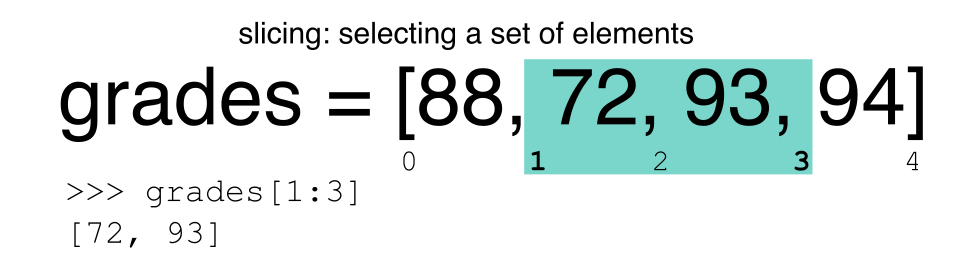
Slicing using the [] operator selects a set of rows and/or columns from a
DataFrame. To slice out a set of rows, you use the following syntax:
data[start:stop]. When slicing in pandas the start bound is included in the
output. The stop bound is one step BEYOND the row you want to select. So if you
want to select rows 0, 1 and 2 your code would look like this:
# Select rows 0, 1, 2 (row 3 is not selected)
waves_df[0:3]
The stop bound in Python is different from what you might be used to in languages like Matlab and R.
# Select the first 5 rows (rows 0, 1, 2, 3, 4)
waves_df[:5]

# Select the last element in the list
# (the slice starts at the last element, and ends at the end of the list)
waves_df[-1:]
Pandas also recognises the step parameter:
# return every other row in the first ten rows
waves_df[0:10:2]
We can also reassign values within subsets of our DataFrame.
But before we do that, let’s look at the difference between the concept of copying objects and the concept of referencing objects in Python.
Copying Objects vs Referencing Objects in Python
Let’s start with an example:
# Using the 'copy() method'
true_copy_waves_df = waves_df.copy()

# Using the '=' operator
ref_waves_df = waves_df
You might think that the code ref_waves_df = waves_df creates a fresh
distinct copy of the waves_df DataFrame object. However, using the =
operator in the simple statement y = x does not create a copy of our
DataFrame. Instead, y = x creates a new variable y that references the
same object that x refers to. To state this another way, there is only
one object (the DataFrame), and both x and y refer to it.
In contrast, the copy() method for a DataFrame creates a true copy of the
DataFrame.
Let’s look at what happens when we reassign the values within a subset of the DataFrame that references another DataFrame object:
# Assign the value `0` to the first three rows of data in the DataFrame
ref_waves_df[0:3] = 0
Let’s try the following code:
# ref_waves_df was created using the '=' operator
ref_waves_df.head()

# true_copy_waves_df was created using the copy() function
true_copy_waves_df.head()

# waves_df is the original dataframe
waves_df.head()
What is the difference between these three dataframes?
When we assigned the first 3 rows the value of 0 using the
ref_waves_df DataFrame, the waves_df DataFrame is modified too.
Remember we created the reference ref_waves_df object above when we did
ref_waves_df = waves_df. Remember waves_df and ref_waves_df
refer to the same exact DataFrame object. If either one changes the object,
the other will see the same changes to the reference object.
However - true_copy_waves_df was created via the copy() function.
It retains the original values for the first three rows.
To review and recap:
-
Copy uses the dataframe’s
copy()methodtrue_copy_waves_df = waves_df.copy() -
A Reference is created using the
=operatorref_waves_df = waves_df
Inserting columns
You can insert a column of data by specifying a column name that doesn’t already exist and passing a list of the same length as the number of rows; e.g.
waves_df["new_column"] = range(0,2073)
Okay, that’s enough of that. Let’s create a brand new clean dataframe from the original data CSV file.
waves_df = pd.read_csv("data/waves.csv")
Slicing Subsets of Rows and Columns in Python
We can select specific ranges of our data in both the row and column directions using either label or integer-based indexing.
locis primarily label based indexing. Integers may be used but they are interpreted as a label.ilocis primarily integer based indexing
Our dataset has labels for columns, but indexes for rows.
To select a subset of rows and columns from our DataFrame, we can use the
iloc method. For example, for the first 3 rows, we can select record_id, name, and date (columns 0, 2,
and 3 when we start counting at 0), like this:
# iloc[row slicing, column slicing]
waves_df.iloc[0:3, [0,2,3]]
which gives the output
  record_id                             Name                Date
0         1  SW Isles of Scilly WaveNet Site    17/04/2023 00:00
1         2         Hayling Island Waverider    17/04/2023 00:00
2         3      Firth of Forth WaveNet Site    17/04/2023 00:00
Notice that we asked for a slice from 0:3. This yielded 3 rows of data. When you ask for 0:3, you are actually telling Python to start at index 0 and select rows 0, 1, 2 up to but not including 3.
Let’s explore some other ways to index and select subsets of data:
# Select all columns for rows of index values 0 and 10
waves_df.loc[[0, 10], :]

# What does this do?
waves_df.loc[0, ['buoy_id', 'record_id', 'Wave Height']]

# What happens when you type the code below?
waves_df.loc[[0, 10, 35549], :]
NOTE 1: with our dataset, we are using integers even when using loc because our DataFrame index
(which is the unnamed first column) is composed of integers - but Pandas converts these to strings. If you had a column of
strings that you wanted to index using labels, you need to convert that columun using the set_index function
NOTE 2: Labels must be found in the DataFrame or you will get a KeyError.
Indexing by labels loc differs from indexing by integers iloc.
With loc, both the start bound and the stop bound are inclusive. When using
loc, integers can be used, but the integers refer to the
index label and not the position. For example, using loc and select 1:4
will get a different result than using iloc to select rows 1:4.
We can also select a specific data value using a row and
column location within the DataFrame and iloc indexing:
# Syntax for iloc indexing to finding a specific data element
dat.iloc[row, column]
In this iloc example,
waves_df.iloc[2, 6]
gives the output
4.5
Remember that Python indexing begins at 0. So, the index location [2, 6] selects the element that is 3 rows down and 7 columns over (Tpeak) in the DataFrame.
It is worth noting that:
- using
locwith a single list of labels (if the rows are labelled) returns rows - using
ilocwith a single list of integers also returns rows
but
- indexing a data frame directly with labels will select columns (e.g.
waves_df[['buoy_id', 'Name', 'Temperature']]), while ranges of integers will select rows (e.g. waves_df[0:13])
Passing a single integer when trying to index a dataframe will raise an error.
Similarly, direct indexing of rows is redundant with using loc, and will raise a KeyError if a single integer or list is used:
# produces an error - even though you might think it looks sensible
waves_df.loc[1:10,1]

# instead, use this:
waves_df.loc[1:10, "buoy_id"]

# or
waves_df.iloc[1:10, 1]
the error will also occur if index labels are used without loc (or column labels used
with it).
A useful rule of thumb is the following:
- integer-based slicing of rows is best done with
ilocand will avoid errors - it is generally consistent with indexing of Numpy arrays) - label-based slicing of rows is done with
loc - slicing of columns by directly indexing column names.
Challenge - Range
What happens when you execute:
waves_df[0:3]waves_df[0]waves_df[:4]waves_df[:-1]What happens when you call:
waves_df.iloc[0:3]waves_df.iloc[0]waves_df.iloc[:4, :]waves_df.iloc[0:4, 1:4]waves_df.loc[0:4, 1:4]
- How are the last two commands different?
Solution
1.
waves_df[0:3]returns the first three rows of the DataFrame:record_id buoy_id Name Date Tz ... Temperature Spread Operations Seastate Quadrant 0 1 14 SW Isles of Scilly WaveNet Site 17/04/2023 00:00 7.2 ... 10.8 26.0 crew swell west 1 2 7 Hayling Island Waverider 17/04/2023 00:00 4.0 ... 10.2 14.0 crew swell south 2 3 5 Firth of Forth WaveNet Site 17/04/2023 00:00 3.7 ... 7.8 28.0 crew windsea east [3 rows x 13 columns]
waves_df[0]results in a ‘KeyError’, since direct indexing of a row is redundant this way -ilocshould be used instead (waves_df[0:1]could be used to obtain only the first row using this notation)
waves_df[:4]slices from the first row to the fourth:record_id buoy_id Name Date Tz ... Temperature Spread Operations Seastate Quadrant 0 1 14 SW Isles of Scilly WaveNet Site 17/04/2023 00:00 7.2 ... 10.8 26.0 crew swell west 1 2 7 Hayling Island Waverider 17/04/2023 00:00 4.0 ... 10.2 14.0 crew swell south 2 3 5 Firth of Forth WaveNet Site 17/04/2023 00:00 3.7 ... 7.8 28.0 crew windsea east 3 4 3 Chesil Waverider 17/04/2023 00:00 5.5 ... 10.2 48.0 crew swell south
waves_df[:-1]provides everything except the final row of a DataFrame. You can use negative index numbers to count backwards from the last entry.2.
waves_df.iloc[0:1]returns the first rowwaves_df.iloc[0]returns the first row as a named listwaves_df.iloc[:4, :]returns all columns of the first four rowswaves_df.iloc[0:4, 1:4]selects specified columns of the first four rowswaves_df.loc[0:4, 1:4]results in a ‘TypeError’ - see below.While
ilocuses integers as indices and slices accordingly,locworks with labels. It is like accessing values from a dictionary, asking for the key names. Column names 1:4 do not exist, so the call tolocabove results in an error. Check also the difference betweenwaves_df.loc[0:4]andwaves_df.iloc[0:4].
Subsetting Data using Criteria
We can also select a subset of our data using criteria. For example, we can select all rows that have a temperature less than or equal to 10 degrees
waves_df[waves_df.Temperature <= 10]
Which produces the following output:
    record_id    buoy_id                Name                Date     Tz    Peak Direction    Tpeak    Wave Height    Temperature    Spread    Operations    Seastate    Quadrant
3           4	         3    Chesil Waverider    17/04/2023 00:00    5.5             225.0      8.3           0.50          10.20      48.0          crew       swell       south
10         11          3    Chesil Waverider    15/04/2023 00:00    3.2             260.0      3.4           0.21           8.95      67.0          crew     windsea        west
Or, we can select all rows that have a buoy_id of 3:
waves_df[waves_df.buoy_id == 3]
We can also select all rows that do not contain values for Tpeak (listed as NaN):
waves_df[waves_df["Tpeak"].isna()]
Or we can select all rows that do not contain the buoy_id 3:
waves_df[waves_df.buoy_id != 3]
We can define sets of criteria too, for example selecting only waves with a height between 3.0 and 4.0 metres:
waves_df[(waves_df["Wave Height"] >= 3.0) & (waves_df["Wave Height"] < 4.0)]
Different types of and
In Python, we can normally use the keyword
andfor the boolean and operator:x = True y = True x and yTruex = True y = False x and yFalseBut, in Pandas we need to use the
&symbol instead. Theandoperator requires boolean values on both sides, but the boolean value of aSeriesis considered ambiguous, and trying to useandreturns an error.
Python Syntax Cheat Sheet
We can use the syntax below when querying data by criteria from a DataFrame. Experiment with selecting various subsets of the “waves” data.
- Equals:
== - Not equals:
!= - Greater than, less than:
>or< - Greater than or equal to
>= - Less than or equal to
<=
Challenge - Queries
Select a subset of rows in the
waves_dfDataFrame that contain data from the year 2023 and that contain Temperature values less than or equal to 8. How many rows did you end up with? Tip #1: You can’t access attributes of a DateTime objects stored in a Series directly! Tip #2: you may want to create a new column containing the dates formatted as DateType that we created earlier!You can use the
isincommand in Python to query a DataFrame based upon a list of values as follows:waves_df[waves_df['buoy_id'].isin([listGoesHere])]Use the
isinfunction to find all plots that contain buoy ids 5 and 7 in the “waves” DataFrame. How many records contain these values?
Experiment with other queries. e.g. Create a query that finds all rows with a Tpeak greater than or equal to 10.
The
~symbol in Python can be used to return the OPPOSITE of the selection that you specify in Python. It is equivalent to is not in. Write a query that selects all rows with Quadrant NOT equal to ‘south’ or ‘east’ in the “waves” data.Solution
This is possible in one-line:
waves_df[(pd.to_datetime(waves_df.Date, format="%d/%m/%Y %H:%M").dt.year == 2023) & (waves_df["Temperature"] <= 8)]First, we convert the
Datecolumn to objects of typeTimestamp, then use thedtaccessor object to get information about the dates. Aseriesisn’t aTimestamp, so we can’t use theTimestampattributes directly. If we wanted to save just the Year in a new column, we could do:timestamps = pd.to_datetime(waves_df.Date, format="%d/%m/%Y %H:%M") years = timestamps.dt.year waves_df["Year"] = years waves_df[(waves_df.Year == 2023) & (waves_df.Temperature <=8)]And then we can see there are 2 rows which match this condition (don’t forget we can also use the
lenfunction)record_id buoy_id Name Date Tz Peak Direction ... Temperature Spread Operations Seastate Quadrant Year 2 3 5 Firth of Forth WaveNet Site 17/04/2023 00:00 3.7 115.0 ... 7.80 28.0 crew windsea east 2023 9 10 5 Firth of Forth WaveNet Site 15/04/2023 00:00 3.2 124.0 ... 7.35 23.0 crew windsea east 2023 [2 rows x 14 columns]waves_df[waves_df['buoy_id'].isin([5,7])]record_id buoy_id Name Date Tz ... Spread Operations Seastate Quadrant Year 1 2 7 Hayling Island Waverider 17/04/2023 00:00 4.0 ... 14.0 crew swell south 2023 2 3 5 Firth of Forth WaveNet Site 17/04/2023 00:00 3.7 ... 28.0 crew windsea east 2023 8 9 7 Hayling Island Waverider 15/04/2023 00:00 3.7 ... 31.0 crew windsea east 2023 9 10 5 Firth of Forth WaveNet Site 15/04/2023 00:00 3.2 ... 23.0 crew windsea east 2023 1071 1072 5 Firth of Forth WaveNet Site 16/02/2009 11:00 3.0 ... 30.0 crew windsea west 2009 ... ... ... ... ... ... ... ... ... ... ... ... 1350 1351 5 Firth of Forth WaveNet Site 22/02/2009 06:30 2.6 ... 16.0 crew windsea west 2009 1351 1352 5 Firth of Forth WaveNet Site 22/02/2009 07:00 2.7 ... 16.0 crew windsea west 2009 1352 1353 5 Firth of Forth WaveNet Site 22/02/2009 07:30 2.7 ... 16.0 crew windsea west 2009 1353 1354 5 Firth of Forth WaveNet Site 22/02/2009 08:00 2.7 ... 12.0 crew windsea west 2009 1354 1355 5 Firth of Forth WaveNet Site 22/02/2009 08:30 2.8 ... 12.0 crew windsea west 2009 [288 rows x 14 columns]len(waves_df[waves_df['buoy_id'].isin([5,7])])5waves_df[waves_df['Tpeak'] >= 10]waves_df[~waves_df['Quadrant'].isin(['south','east'])]record_id buoy_id Name Date Tz ... Spread Operations Seastate Quadrant Year 0 1 14 SW Isles of Scilly WaveNet Site 17/04/2023 00:00 7.2 ... 26.0 crew swell west 2023 4 5 10 M6 Buoy 17/04/2023 00:00 7.6 ... 89.0 no go swell west 2023 5 6 9 Lomond 17/04/2023 00:00 4.0 ... NaN crew swell north 2023 6 7 2 Cardigan Bay 17/04/2023 00:00 5.9 ... 18.0 crew swell west 2023 7 8 14 SW Isles of Scilly WaveNet Site 15/04/2023 00:00 7.2 ... 18.0 crew swell west 2023 ... ... ... ... ... ... ... ... ... ... ... ... 2068 2069 16 west of Hebrides 18/10/2022 16:00 6.1 ... 28.0 crew swell north 2022 2069 2070 16 west of Hebrides 18/10/2022 16:30 5.9 ... 34.0 crew swell north 2022 2070 2071 16 west of Hebrides 18/10/2022 17:00 5.6 ... 34.0 crew swell north 2022 2071 2072 16 west of Hebrides 18/10/2022 17:30 5.7 ... 31.0 crew swell north 2022 2072 2073 16 west of Hebrides 18/10/2022 18:00 5.7 ... 34.0 crew swell north 2022 [1985 rows x 14 columns]
Using masks to identify a specific condition
A mask can be useful to locate where a particular subset of values exist or
don’t exist - for example, NaN, or “Not a Number” values. To understand masks,
we also need to understand bool objects in Python.
Boolean values are either True or False. For example,
# Set x to 5
x = 5

# What does the code below return?
x > 5

# How about this?
x == 5
When we ask Python whether x is greater than 5, it returns False.
This is Python’s way to say “No”. Indeed, the value of x is 5,
and 5 is not greater than 5.
To create a boolean mask:
- Set the True / False criteria (e.g.
values > 5) - Python will then assess each value in the object to determine whether the value meets the criteria (True) or not (False).
- Python creates an output object that is the same shape as the original
object, but with a
TrueorFalsevalue for each index location.
Let’s try this out. Let’s identify all locations in the wave data that have
null (missing or NaN) data values. We can use the isnull method to do this.
The isnull method will compare each cell with a null value. If an element
has a null value, it will be assigned a value of True in the output object.
pd.isnull(waves_df)
A snippet of the output is below:
    record_id    buoy_id     Name     Date       Tz    Peak Direction    Tpeak    Wave Height    Temperature    Spread    Operations    Seastate    Quadrant
0       False      False    False    False    False             False    False          False          False     False         False       False       False
1       False      False    False    False    False             False    False          False          False     False         False       False       False
2       False      False    False    False    False             False    False          False          False     False         False       False       False
To select the rows where there are null values, we can use the mask as an index to subset our data as follows:
# To select just the rows with NaN values, we can use the 'any()' method
waves_df[pd.isnull(waves_df).any(axis=1)]
Note that the Temperature and other columns of our DataFrame contains many null or NaN
values. Remember we’ve disucssed ways of dealing with this in the previous episode on Data Types and Formats.
As we saw earlier, we can run isnull on a particular column too. What does the code below do?
# What does this do?
waves_df[pd.isnull(waves_df['Temperature'])]['Temperature']
Let’s take a minute to look at the statement above. We are using the bool
array pd.isnull(waves_df['Temperature']) as an index to waves_df. We are
asking Python to select rows that have a NaN value of Temperature.
Challenge - Putting it all together
Create a new DataFrame that only contains observations with Operations values that are not crew or survey. Print the number of rows in this new DataFrame. Verify the result by comparing the number of rows in the new DataFrame with the number of rows in the waves DataFrame where Site Type is No Go.
Create a new DataFrame that contains only observations from the Chesil Waverider or Hayling Island Waverider buoys, and where the wave height is less than 50 cm.
Create a new DataFrame that contains only observations that are of Quadrant north or west and where Tpeak values are greater than 10.
Solution
# 1.
waves_df[
  ~waves_df["Operations"].isin(["crew", "survey"])
]

# 2.
waves_df[
  waves_df.Name.isin(["Chesil Waverider", "Hayling Island Waverider"]) &
  (waves_df['Wave Height'] < 0.5)
]

# 3.
waves_df[
  waves_df.Quadrant.isin(["north", "west"]) &
  (waves_df.Tpeak > 10)
]

# Alternative for 3.
waves_df[(waves_df["buoy_id"].isin([3,7])) & (waves_df["Wave Height"] < 0.5)]
Key Points
In Python, portions of data can be accessed using indices, slices, column headings, and condition-based subsetting.
Python uses 0-based indexing, in which the first element in a list, tuple or any other data structure has an index of 0.
Pandas enables common data exploration steps such as data indexing, slicing and conditional subsetting.
Combining DataFrames with Pandas
Overview
Teaching: 20 min
Exercises: 25 minQuestions
Can I work with data from multiple sources?
How can I combine data from different data sets?
Objectives
Combine data from multiple files into a single DataFrame using merge and concat.
Combine two DataFrames using a unique ID found in both DataFrames.
Employ
to_csvto export a DataFrame in CSV format.Join DataFrames using common fields (join keys).
In many “real world” situations, the data that we want to use come in multiple
files. We often need to combine these files into a single DataFrame to analyze
the data. The pandas package provides various methods for combining
DataFrames including
merge and concat.
To work through the examples below, we first need to load the file which contains our waves data and also two additional files which contains information about the buoys:
import pandas as pd
waves_df = pd.read_csv("data/waves.csv",
                         keep_default_na=False, na_values=[""])
waves2020_df = pd.read_csv("data/waves_2020.csv",
                         keep_default_na=False, na_values=[""])
buoys_df = pd.read_csv("data/buoy_data.csv",
                         keep_default_na=False, na_values=[""])
Take note that the read_csv method we used can take some additional options which
we didn’t use previously. Many functions in Python have a set of options that
can be set by the user if needed. In this case, we have told pandas to assign
empty values in our CSV to NaN keep_default_na=False, na_values=[""].
We have explicitly requested to change empty values in the CSV to NaN,
this is however also the default behaviour of read_csv.
More about all of the read_csv options here and their defaults.
Concatenating DataFrames
We can use the concat function in pandas to append either columns or rows from
one DataFrame to another. waves2020_df contains data from the year 2020,
and which is in the same format as our waves_df to see how this works.
# Now read in first 8 lines of the waves 2020 data
waves_sub = waves2020_df.head(8)
# Grab the last 8 rows
waves_sub_last8 = waves2020_df.tail(8)
# Reset the index values to the second dataframe
waves_sub_last8 = waves_sub_last8.reset_index(drop=True)
# drop=True option avoids adding new index column with old index values
# Have a look at waves_sub_last8 to see the effect
When we concatenate DataFrames, we need to specify the axis. axis=0 tells
pandas to stack the second DataFrame UNDER the first one. It will automatically
detect whether the column names are the same and will stack accordingly.
axis=1 will stack the columns in the second DataFrame to the RIGHT of the
first DataFrame. To stack the data vertically, we need to make sure we have the
same columns and associated column format in both datasets. When we stack
horizontally, we want to make sure what we are doing makes sense (i.e. the data are
related in some way).
# Stack the DataFrames on top of each other
vertical_stack = pd.concat([waves_sub, waves_sub_last8], axis=0)

# Place the DataFrames side by side
horizontal_stack = pd.concat([waves_sub, waves_sub_last8], axis=1)
Row Index Values and Concat
Have a look at the vertical_stack dataframe? Notice anything unusual?
The row indexes for the two data frames waves_sub and waves_sub_last8
have been repeated. We can reindex the new dataframe using the reset_index() method.
Writing Out Data to CSV
We can use the to_csv command to do export a DataFrame in CSV format. Note that the code
below will by default save the data into the current working directory. We can
save it to a different folder by adding the foldername and a slash to the file
vertical_stack.to_csv('foldername/out.csv'). We use the ‘index=False’ so that
pandas doesn’t include the index number for each line.
# Write DataFrame to CSV
vertical_stack.to_csv('data/out.csv', index=False)
Check out your working directory to make sure the CSV wrote out properly, and that you can open it! If you want, try to bring it back into Python to make sure it imports properly.
# For kicks read our output back into Python and make sure all looks good
new_output = pd.read_csv('data/out.csv', keep_default_na=False, na_values=[""])
Challenge - Combine Data
In the data folder, there are two waves data files:
waves.csvandwaves_2020.csv. Read the data into Python and combine the files to make one new data frame. Output some descriptive statistics group by buoy_id. Export your results as a CSV and make sure it reads back into Python properly.Solution
# read the files
waves_df = pd.read_csv("waves.csv", keep_default_na=False, na_values=[""])
waves2020_df = pd.read_csv("waves_2020.csv", keep_default_na=False, na_values=[""])
# concatenate
combined_data = pd.concat([waves_df, waves2020_df], axis=0)
# group by buoy_id, and output some summary statistics
combined_data.groupby("buoy_id").describe()
# write to csv
combined_data.to_csv("combined_wave_data.csv", index=False)
# read in the csv
cwd = pd.read_csv("combined_wave_data.csv", keep_default_na=False, na_values=[""])
# check the results are the same
cwd.groupby("buoy_id").describe()
Joining DataFrames
When we concatenated our DataFrames we simply added them to each other - stacking them either vertically or side by side. Another way to combine DataFrames is to use columns in each dataset that contain common values (a common unique id). Combining DataFrames using a common field is called “joining”. The columns containing the common values are called “join key(s)”. Joining DataFrames in this way is often useful when one DataFrame is a “lookup table” containing additional data that we want to include in the other.
NOTE: This process of joining tables is similar to what we do with tables in an SQL database.
For example, the buoys_data.csv file that we’ve been working with could be considered as a “lookup”
table. This table contains the data for 15 buoys. This new table details
where the buoy is (Country, Site Type, latitude and longitude), as well as water
depth and information about the observing platform (Manufacturer, Type, operator)
The Name and buoy_id code are unique for each line. These buoys are identified in our waves
data as well using the buoy_id (and more memorable ‘Name’). Rather than adding 8 more
columns to include these data to each of the multiple lines in the waves data and waves_2020 tables, we
can maintain the shorter table with the buoy information. When we want to
access that information, we can create a query that joins the additional columns
of information to the waves data.
Storing data in this way has many benefits including:
- It ensures consistency in the spelling of buoy attributes (site name, manufacturer etc.) given each buoy is only entered once. Imagine the possibilities for spelling errors when copying the data thousands of times!
- It also makes it easy for us to make changes or add information about the buoys once without having to find each instance of it in the larger wave observations data.
- It optimizes the size of our data.
Joining Two DataFrames
To better understand joins, let’s grab the first 10 lines of our data as a
subset to work with. We’ll again use the .head method to do this. We’ll also read
in the meta data for the buoys ‘buoys_data.csv’ as a look-up table.
# Read in first 10 lines of waves table
wave_sub = waves_df.head(10)
We’ve already read in buoys_df, which is the table containing buoy names and information
that we want to join with the data in wave_sub to produce a new
DataFrame that contains all of the columns from both buoys_df and
waves_df.
Identifying join keys
To identify appropriate join keys we first need to know which field(s) are shared between the files (DataFrames). We might inspect both DataFrames to identify these columns. If we are lucky, both DataFrames will have columns with the same name that also contain the same data. If we are less lucky, we need to identify a (differently-named) column in each DataFrame that contains the same information.
>>> buoys_df.columns

Index(['buoy_id', 'Name', 'Manufacturer', 'Depth', 'Type', 'operator',
       'Country', 'Site Type', 'latitude', 'longitude'],
      dtype='object')

>>> wave_sub.columns
Index(['record_id', 'buoy_id', 'Name', 'Date', 'Tz', 'Peak Direction', 'Tpeak',
       'Wave Height', 'Temperature', 'Spread', 'Operations', 'Seastate',
       'Quadrant'],
      dtype='object')
In our example, the join key is the column containing the buoy_id.
Now that we know the fields with the common buoy_id attributes in each
DataFrame, we are almost ready to join our data. However, since there are
different types of joins, we
also need to decide which type of join makes sense for our analysis.
Inner joins
The most common type of join is called an inner join. An inner join combines two DataFrames based on a join key and returns a new DataFrame that contains only those rows that have matching values in both of the original DataFrames.
Inner joins yield a DataFrame that contains only rows where the value being joined exists in BOTH tables. An example of an inner join, adapted from Jeff Atwood’s blogpost about SQL joins is below:

The pandas function for performing joins is called merge and an Inner join is
the default option:
merged_inner = pd.merge(left=wave_sub, right=buoys_df, left_on='buoy_id', right_on='buoy_id')
# In this case `buoy_id` is the only column name in  both dataframes, so if we skipped `left_on`
# And `right_on` arguments we would still get the same result

# What's the size of the output data?
merged_inner.shape
(9, 22)
The result of an inner join of wave_sub and buoys_df is a new DataFrame
that contains the combined set of columns from wave_sub and buoys_df. It
only contains rows that have buoy ID that are the same in
both the wave_sub and buoys_df DataFrames. In other words, if a row in
wave_sub has a value of buoy_id that does not appear in the buoy_id
column of buoys_data, it will not be included in the DataFrame returned by an
inner join. Similarly, if a row in buoys_df has a value of buoy_id
that does not appear in the buoy_id column of wave_sub, that row will not
be included in the DataFrame returned by an inner join. In our example, there is
data from the M6 Buoy, but this buoy (id 10) does not exist in our buoy data.
The two DataFrames that we want to join are passed to the merge function using
the left and right argument. The left_on='buoy_id' argument tells merge
to use the buoy_id column as the join key from wave_sub (the left
DataFrame). Similarly , the right_on='buoy_id' argument tells merge to
use the buoy_id column as the join key from buoys_df (the right
DataFrame). For inner joins, the order of the left and right arguments does
not matter.
The result merged_inner DataFrame contains all of the columns from wave_sub
(record id, Tz, Peak Direction, Tpeak, etc.) as well as all the columns from
buoys_df (buoy_id, Name, Manufacturer, Depth, Type, operator, Country, Site,
Type, latitude, and longitude).
Notice that merged_inner has fewer rows than wave_sub. This is an
indication that there were rows in waves_df with value(s) for buoy_id that
do not exist as value(s) for buoy_id in buoys_df.
Left joins
What if we want to add information from buoys_df to wave_sub without
losing any of the information from wave_sub? In this case, we use a different
type of join called a “left outer join”, or a “left join”.
Like an inner join, a left join uses join keys to combine two DataFrames. Unlike
an inner join, a left join will return all of the rows from the left
DataFrame, even those rows whose join key(s) do not have values in the right
DataFrame. Rows in the left DataFrame that are missing values for the join
key(s) in the right DataFrame will simply have null (i.e., NaN or None) values
for those columns in the resulting joined DataFrame.
Note: a left join will still discard rows from the right DataFrame that do not
have values for the join key(s) in the left DataFrame.
A left join is performed in pandas by calling the same merge function used for
inner join, but using the how='left' argument:
merged_left = pd.merge(left=wave_sub, right=buoys_df, how='left', left_on='buoy_id', right_on='buoy_id')
merged_left
The result DataFrame from a left join (merged_left) looks very much like the
result DataFrame from an inner join (merged_inner) in terms of the columns it
contains. However, unlike merged_inner, merged_left contains the same
number of rows as the original wave_sub DataFrame. When we inspect
merged_left, we find there are rows where the information that should have
come from buoys_df (i.e. buoy_id, Name, Manufacturer, Depth, Type, operator,
Country, Site, Type, latitude, and longitude). is missing (they contain NaN values):
merged_left[ pd.isnull(merged_left.Name_y) ]
These rows are the ones where the value of buoy_id from wave_sub (in this
case, M6 Buoy) does not occur in buoys_df. Also note that where the two
DataFrames have columns with the same name, Pandas appends _x to the column
from the “left” dataframe, and _y to the column from the “right” dataframe.
Other join types
The pandas merge function supports two other join types:
- Right (outer) join: Invoked by passing
how='right'as an argument. Similar to a left join, except all rows from therightDataFrame are kept, while rows from theleftDataFrame without matching join key(s) values are discarded. - Full (outer) join: Invoked by passing
how='outer'as an argument. This join type returns the all pairwise combinations of rows from both DataFrames; i.e., the result DataFrame willNaNwhere data is missing in one of the dataframes. This join type is very rarely used.
Final Challenges
Challenge - Distributions
Create a new DataFrame by joining the contents of the
waves.csvandbuoys_data.csvtables. Then calculate the mean:
- Wave Height by Site Type
- Temperature by Seastate and by Country
Solution
# Merging the data frames
merged_left = pd.merge(left=waves_df,right=buoys_df, how='left', on="buoy_id")
# Group by Site Type, and calculate mean of Wave Height
merged_left.groupby("Type")["Wave Height"].mean()
# Group by Sea State and Country, and calculate mean of Temperature
merged_left.groupby(["Seastate","Country"])["Temperature"].mean()
Type Directional 3.489321 Downward-looking wave radar 0.600000 Unspecified wave measurement sensor 0.381098 Name: Wave Height, dtype: float64Seastate Country swell England 17.324093 Scotland 10.935880 Wales 12.491667 windsea England 9.300000 Scotland 5.404502 Wales 12.771239 Name: Temperature, dtype: float64
Challenge - filter by availability
- In the data folder, there is a
access.csvfile that contains information about the data availability and access rights associated with each buoy. Use that data to summarize the number of observations which are reusable for research.- Again using
access.csvfile, use that data to summarize the number of data records from operational buoys which are available in Coastal versus Ocean waters.Solution
1.
# Read the access file
access_df = pd.read_csv("data/access.csv")
# Merge the dataframes
merged_access = pd.merge(left=waves_df,right=access, how='left', on="buoy_id")
# find the number available for research
merged_access.groupby("data availability").count()
# or, this also gives the same answer:
merged_access[merged_access["data availability"]=="research"]
2.
buoy_access = pd.merge(left=buoys_df, right=access, how="left", on="buoy_id")
buoy_access[buoy_access["data availability"]=="operational"].groupby("Site Type")["buoy_id"].count()
Key Points
Pandas’
mergeandconcatcan be used to combine subsets of a DataFrame, or even data from different files.
joinfunction combines DataFrames based on index or column.Joining two DataFrames can be done in multiple ways (left, right, and inner) depending on what data must be in the final DataFrame.
to_csvcan be used to write out DataFrames in CSV format.
Data Ingest and Visualization - Matplotlib and Pandas
Overview
Teaching: 40 min
Exercises: 65 minQuestions
What tools can I use to create plots?
Why should I use Python to create plots?
Objectives
Import the pyplot toolbox to create figures in Python.
Use matplotlib to make adjustments to Pandas objects.
Putting it all together
Up to this point, we have walked through tasks that are often involved in handling and processing data using the workshop-ready cleaned files that we have provided. In this wrap-up exercise, we will perform many of the same tasks with real data sets. This lesson also covers data visualization.
As opposed to the previous ones, this lesson does not give step-by-step directions to each of the tasks. Use the lesson materials you’ve already gone through as well as the Python documentation to help you along.
Obtain data
There are many repositories online from which you can obtain data. We are
providing you with one data file to use with these exercises, but feel free to
use any data that is relevant to your research. The file
bouldercreek_09_2013.txt
contains stream discharge data, summarized at
15 minute intervals (in cubic feet per second) for a streamgage on Boulder
Creek at North 75th Street (USGS gage06730200) for 1-30 September 2013. If you’d
like to use this dataset, please download it and put it in your data directory.
Clean up your data and open it using Python and Pandas
To begin, import your data file into Python using Pandas. Did it fail? Your data file probably has a header that Pandas does not recognize as part of the data table. Remove this header, but do not simply delete it in a text editor! Use either a shell script or Python to do this - you wouldn’t want to do it by hand if you had many files to process.
If you are still having trouble importing the data as a table using Pandas, check the documentation. You can open the docstring in a Jupyter Notebook using a question mark. For example:
import pandas as pd
pd.read_csv?
Look through the function arguments to see if there is a default value that is
different from what your file requires (Hint: the problem is most likely the
delimiter or separator. Common delimiters are ',' for comma, ' ' for space,
and '\t' for tab).
Create a DataFrame that includes only the values of the data that are useful to you. In the streamgage file, those values might be the date, time, and discharge measurements. Convert any measurements in imperial units into SI units. You can also change the name of the columns in the DataFrame like this:
df = pd.DataFrame({'1stcolumn':[100,200], '2ndcolumn':[10,20]}) # this just creates a DataFrame for the example!
print('With the old column names:\n') # the \n makes a new line, so it's easier to see
print(df)

df.columns = ['FirstColumn', 'SecondColumn'] # rename the columns!
print('\n\nWith the new column names:\n')
print(df)
With the old column names:

   1stcolumn  2ndcolumn
0        100         10
1        200         20


With the new column names:

   FirstColumn  SecondColumn
0          100            10
1          200            20
Matplotlib package
Matplotlib is a Python package that is widely used throughout the scientific Python community to create high-quality and publication-ready graphics. It supports a wide range of raster and vector graphics formats including PNG, PostScript, EPS, PDF and SVG.
Moreover, matplotlib is the actual engine behind the plotting capabilities of Pandas. For example, as we’ll see, we can call the .plot method on Pandas data objects - this actually uses the matplotlib package. There are also alternative plotting packages, e.g. PLotnine, which is also built upon Matplotlib.
First, import the pyplot toolbox:
import matplotlib.pyplot as plt
Now, let’s read data and plot it!
waves = pd.read_csv("data/waves.csv")
my_plot = waves.plot("Tpeak", "Wave Height", kind="scatter")
plt.show() # not necessary in Jupyter Notebooks
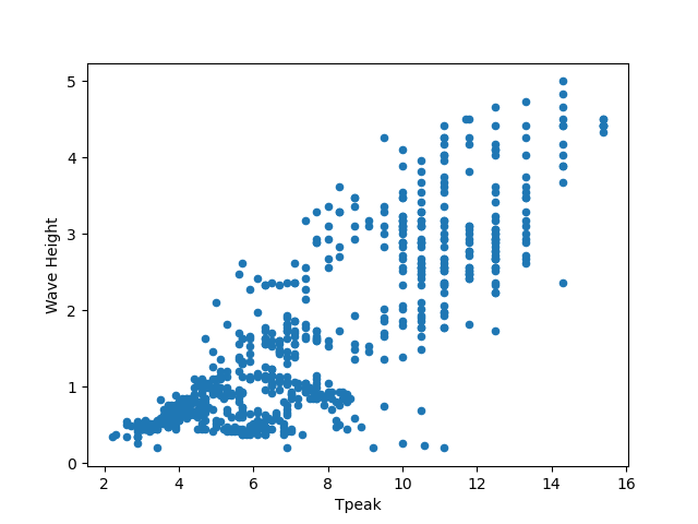
Tip
By default, matplotlib creates a figure in a separate window. When using Jupyter notebooks, we can make figures appear in-line within the notebook by executing:
%matplotlib inline
The returned object is a matplotlib object (check it yourself with type(my_plot)),
to which we may make further adjustments and refinements using other matplotlib methods.
Tip
Matplotlib itself can be overwhelming, so a useful strategy is to do as much as you easily can in a convenience layer, i.e. start creating the plot in Pandas, and then use matplotlib for the rest.
We will cover a few basic commands for creating and formatting plots with matplotlib in this lesson. A great resource for help creating and styling your figures is the matplotlib gallery (http://matplotlib.org/gallery.html), which includes plots in many different styles and the source codes that create them.
plt pyplot versus object-based matplotlib
Matplotlib integrates nicely with the NumPy package and can use NumPy arrays as input to the available plot functions. Consider the following example data, created with NumPy by drawing 1000 samples from a normal distribution with a mean value of 0 and a standard deviation of 0.1:
import numpy as np
sample_data = np.random.normal(0, 0.1, 1000)
To plot a histogram of our draws from the normal distribution, we can use the hist function directly:
plt.hist(sample_data)
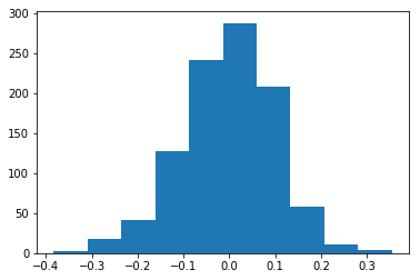
Tip: Cross-Platform Visualization of Figures
Jupyter Notebooks make many aspects of data analysis and visualization much simpler. This includes doing some of the labor of visualizing plots for you. But, not every one of your collaborators will be using a Jupyter Notebook. The
.show()command allows you to visualize plots when working at the command line, with a script, or at the IPython interpreter. In the previous example, addingplt.show()after the creation of the plot will enable your colleagues who aren’t using a Jupyter notebook to reproduce your work on their platform.
or create matplotlib figure and axis objects first and subsequently add a histogram with 30
data bins:
fig, ax = plt.subplots()  # initiate an empty figure and axis matplotlib object
ax.hist(sample_data, 30)
Although the latter approach requires a little bit more code to create the same plot, the advantage is that it gives us full control over the plot and we can add new items such as labels, grid lines, title, and other visual elements. For example, we can add additional axes to the figure and customize their labels:
# prepare a matplotlib figure
fig, ax1 = plt.subplots()
ax1.hist(sample_data, 30)
# add labels
ax1.set_ylabel('density')
ax1.set_xlabel('value')

# define and sample beta distribution
a = 5
b = 10
beta_draws = np.random.beta(a, b)

# add additional axes to the figure to plot beta distribution
ax2 = fig.add_axes([0.125, 0.575, 0.3, 0.3])  # number coordinates correspond to left, bottom, width, height, respectively
ax2.hist(beta_draws)
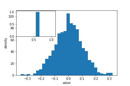
Challenge - Drawing from distributions
Have a look at
numpy.randomdocumentation. Choose a distribution you have no familiarity with, and try to sample from and visualize it.
Link matplotlib and Pandas
When we create a plot using pandas (or plotnine), it uses matplotlib to create those plots. The plots created in pandas or plotnine are matplotlib objects, which enables us to use some of the advanced plotting options available in the matplotlib library. Because the objects output by pandas and plotnine can be read by matplotlib, we have many more options than any one library can provide, offering a consistent environment to make publication-quality visualizations.
fig, ax1 = plt.subplots() # prepare a matplotlib figure

waves.plot("Tpeak", "Wave Height", kind="scatter", ax=ax1)

# Provide further adaptations with matplotlib:
ax1.set_xlabel("Tpeak (highest energy wave periodicity; seconds)")
ax1.tick_params(labelsize=16, pad=8)
ax1.set_ylabel("Significant Wave Height (metres)")
fig.suptitle('Scatter plot of Significant Wave Height versus Tpeak', fontsize=15)
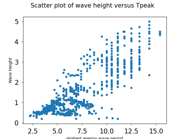
More complicated plotting
What about plotting after joining DataFrames? Let’s plot the water depths at each of the buoys
# water depth in the buoys dataframe is currently a string (it's suffixed by "m") so we need to fix that
def fix_depth_string(i, depth):
    if type(depth) == str:
        buoys_df["Depth"][i] = float((buoys_df["Depth"][i]).strip().rstrip("m"))

for i, depth in enumerate(buoys_df["Depth"]):
    fix_depth_string(i, depth)

joined = pd.merge(left=waves_df, right=buoys_df, left_on='buoy_id', right_on='buoy_id')
plt.bar(joined["Name_x"].unique(), joined["Depth"].unique())
Notice that we have to use Name_x: where column names are duplicated between DataFrames, Pandas
appends _x to the column name that came from the “left”, and _y to the column name that came from
the “right”.
We can plot only the non-null values:
names = joined["Name_x"].unique()
depths = joined["Depth"].unique()
depths_df = pd.DataFrame({"depths":depths, "names":names})
depths_df = depths_df[~depths_df["depths"].isna()]
plt.bar(depths_df["names"], depths_df["depths"])
Note that the return type of .unique is a Numpy ndarray, even though the column were of type Series!
Challenge - subsetting data before plotting
Plot Tpeak vs Wave Height from the West Hebrides site. Can you add appropriate labels and a title, and Make both axes start at 0?
Answers
fig, ax1 = plt.subplots()
waves[waves["buoy_id"] == 16].plot("Tpeak", "Wave Height", kind="scatter", ax=ax1)
ax1.set_xlabel("Highest energy wave period")
ax1.tick_params(labelsize=16, pad=8)
ax1.set_xbound(0, waves[waves["buoy_id"] == 16].Tpeak.max()+1)
ax1.set_ybound(0, waves[waves["buoy_id"] == 16]["Wave Height"].max()+1)
fig.suptitle('Scatter plot of wave height versus Tpeak for West Hebrides', fontsize=15)
Challenge - grouping data before plotting
Can you group the waves data by buoy id, find only the maximum value for wave height for each buoy, and then plot Temperature vs Wave Height for these values. Is there more useful information you could add to this plot?
Answers
data = waves.groupby("buoy_id").max("Wave Height")
x = data["Temperature"]
y = data["Wave Height"]
fig, plot = plt.subplots() # although we're not using the `fig` variable, subplots returns 2 objects
plot.scatter(x, y) # notice a different way of creating a scatter plot
for i in data.index:
    plot.annotate(i, (x[i], y[i]), xytext=(5, -5), textcoords="offset pixels") # annotate the point with the buoy index
Challenge - multiple datasets
Plot Wave Height vs Tpeak for both the West Hebrides and the South Pembrokeshore buoys. Change the marker style for one of the Series, and make sure that you include a legend
Answers
fig, ax = plt.subplots()
wh = waves[waves["buoy_id"] == 16]
pb = waves[waves["buoy_id"] == 11]

ax.scatter(wh["Tpeak"], wh["Wave Height"])
ax.scatter(pb["Tpeak"], pb["Wave Height"], marker="*")

ax.legend(["West Hebrides", "South Pembrokeshire"], loc="best")
Saving matplotlib figures
Once satisfied with the resulting plot, you can save the plot with the .savefig(*args) method from matplotlib:
fig.savefig("my_plot_name.png")
which will save the fig created using Pandas/matplotlib as a png file with the name my_plot_name
Tip: Saving figures in different formats
Matplotlib recognizes the extension used in the filename and supports (on most computers) png, pdf, ps, eps and svg formats.
Challenge - Saving figure to file
Check the documentation of the
savefigmethod and check how you can comply to journals requiring figures asAnswers
fig.savefig("my_plot_name.pdf", dpi=300)
Make other types of plots:
Matplotlib can make many other types of plots in much the same way that it makes two-dimensional line plots. Look through the examples in
http://matplotlib.org/users/screenshots.html and try a few of them (click on the
“Source code” link and copy and paste into a new cell in Jupyter Notebook or
save as a text file with a .py extension and run in the command line).
Challenge - Final Plot
Display your data using one or more plot types from the example gallery. Which ones to choose will depend on the content of your own data file. If you are using the streamgage file
bouldercreek_09_2013.txt, you could make a histogram of the number of days with a given mean discharge, use bar plots to display daily discharge statistics, or explore the different ways matplotlib can handle dates and times for figures.
Key Points
Matplotlib is the engine behind plotnine and Pandas plots.
The object-based nature of matplotlib plots enables their detailed customization after they have been created.
Export plots to a file using the
savefigmethod.
A brief introduction to geospatial data
Overview
Teaching: 30 min
Exercises: 45 minQuestions
What can I do with geospatial data in Python?
How can I visualise and analyse this data?
Objectives
Import the Geopandas module to analyse latitude / longitude data.
Use Geopandas and Geoplot to help with visualisation.
Geospatial Data
Often in the Environmental Sciences, we need to deal with geospatial data. This is normally presented as latitude and longitude (either as decimal degrees or as degrees/minutes/seconds), but can be presented in other formats (e.g. OSGB for UK Grid References).
A full discussion of geospatial vector data is beyond the scope of this episode - if you need more background please see this Carpentries Incubator lesson. Instead, we will highlight some useful tasks that can achieved with some key python libraries.
We’ll be using the data about buoys again.
import pandas as pd
buoys = pd.read_csv("data/buoy_data.csv",
                         keep_default_na=False, na_values=[""])
We can see that the dataset has a latitude and longitude. Let’s subset this data, along with the names.
locations = buoys[["Name", "latitude", "longitude"]]
To be able to deal with geospatial data, we need a python package that doesn’t come included with the Conda distribution we’re using. We can install the additional packages we need directly within a Notebook:
conda install geopandas -c conda-forge
conda install geoplot -c conda-forge
These might take several minutes to run. Once they’ve been installed, we can import them:
import geopandas as gpd
import geoplot as gplt
Conda environments
We’re now at the stage where you might find it useful to have different python environments for specific tasks. When you open Anaconda Navigator, it will, by default, be running in your
baseenvironment. However, you can create new environments via the Environments tab in the left-hand menu. Each environment can have different packages (or different versions of packages), different versions of python, etc - and different packages can be installed via the Environments tab. However, note that individual Notebooks are not associated with specific environments - they are associated with the current active environment. A full introduction to Conda environments can be found at https://carpentries-incubator.github.io/introduction-to-conda-for-data-scientists/
In our locations DataFrame, latitude and longitude are of type float:
locations.dtypes
Name          object
latitude     float64
longitude    float64
dtype: object
We need to convert the latitude and longitude to geometry data using Geopandas:
buoys_geo = gpd.GeoDataFrame(
    locations, geometry=gpd.points_from_xy(locations.longitude, locations.latitude), crs="EPSG:4326"
)
The value we’ve given to the crs argument specifies that the data is latitude and longitude, rather
than any other coordinate system. We can now see that the buoys_geo DataFrame contains a new column, geometry,
which also has type geometry.
So, what can we do with this data type?
Calculating distances
Calculating distances often involves some error if we need to convert between different coordinate types.
Geopandas includes a distance function, but to calculate a distance in meters, we need to either project
them in a local coordinate system to approximate the distance with a good precision, or use the
Haversine equation (which is more accurate, but not implemented in Geopandas). In our case, we can project
the data to the UK National Grid. The resulting distances will then be in metres:
buoys_geo.to_crs(epsg=27700,inplace=True)
buoys_geo["geometry"].distance(buoys_geo.iloc[0,3])
Notice the espg=27700 argument - this is the ESPG code for the UK National Grid. We have then calculated the
distance of every point relative to the first point in the Series (Beryl A).
For the rest of the lesson, we need to consider the data back in Latitude / Longitude format, so let’s revert it back:
buoys_geo.to_crs(epsg="4326",inplace=True)
Geospatial polygons
In our case, the geospatial data are all individual points. However, geospatial data can also deal with polygons. Let’s load in data about Scottish Local Authority Boundaries:
scotland = gpd.read_file("data/scotland_boundaries.geojson")
We can immediately plot this:
scotland.plot()
We can see it looks like Scotland! We can look at the shape of the DataFrame to see that it has 32 rows - this is the number of Local Authorities in Scotland, and 5 columns.
We can find the “centroid” point of each Polygon - we can even plot this if we want an abstract map of Scotland!
scotland.centroid.plot()
We can also find the boundary length of each polygon. If we create add this to the DataFrame, then we can sort the resulting DataFrame and see which Council area has the shortest boundary:
scotland["lengths"] = scotland.length
scotland.sort_values("lengths")
Now, let’s look at a different geospatial file: the boundaries of the Cairngorms National Park, one of the National Parks in Scotland, and we can plot it
# Notice this is a different file format to the geojson file we used for the Scottish Council Boundaries data
# This is one file which makes up the Shapefile data format. At a minimum, there needs to be corresponding `shx` and `dbf` files (with the same filenames) in the same directory, but `prj`, `sbx`, `sbn`, and `shp.xml` can store additional metadata
cairngorms =  gpd.read_file("data/cairngorms_boundary.shp")
cairngorms.plot()
Challenge: distances
This dataset also contains the length of the boundary, and the area of the National Park. Print these in km and square km, respectively
Solution
cairngorms.length/1000
cairngorms.area/1000000
One advantage of using geospatial data is seeing how things overlap. Geopandas contains an overlap method to
find objects which have some (but not all) points in common. (There is also a similar intersects method.)
The overlap method can compare a single obect with a Series of objects, so let’s see which Scottish areas overlap with
the Cairngorms National Park:
scotland.overlaps(cairngorms.iloc[0].geometry)
Challenge: overlaps
- Subset the Scotland dataset to show only the rows which overlap with the Cairngorms. Can you display only the names?
- Look in the Geopandas documentation (https://geopandas.org/en/stable/index.html) for the
disjointmethod. What do you think it will return when you run it in the way that we ranoverlap? Try it - did you get the expected result? Can you plot this?Solution
overlaps = scotland.overlaps(cairngorms.iloc[0].geometry)
# get a Series of only the overlaps
overlaps = overlaps.where(overlaps == True).dropna().index
OR, more concisely
overlaps = overlaps.index[overlaps]
# use this to subset the Scotland dataframe
scotland.loc[overlaps]
# ...and get the names
scotland.loc[overlaps].local_authority
disjoints = scotland.disjoint(cairngorms.iloc[0].geometry) # get a Series of only the disjoints disjoints = disjoints.index[disjoints] # use this to subset the Scotland dataframe disjoints = scotland.loc[disjoints] disjoints.plot()
Challenge: plotting
We’ve already seen that we plot GeoDataFrames. We can pass these to Matplotlib subplots in the same way as any other figure. Can you plot the Scotland and Cairngorms GeoDataFrames on the same axes, and customise the plot to highlight the Cairngorms data in some way?
Solution
import matplotlib.pyplot as plt
figure, ax = plt.subplots()
scotland.plot(ax=ax)
cairngorms.plot(ax=ax, color="green")
Finally, Geopandas has a method to show geospatial data over an interactive map:
cairngorms.explore(style_kwds={"fillColor":"lime"})
We can even display the Cairngorms data directly over the Scotland plot, which validates that the result of our intersect command was correct
scotland_plot = scotland.explore()
cairngorms.explore(map=scotland_plot, style_kwds={"fillColor":"lime"})
Back to our buoy data
Our buoy data is based around the UK. Geopandas includes some very low resolution maps which we can use to plot our geospatial data on
world = gpd.read_file(gpd.datasets.get_path("naturalearth_lowres"))
ax = world.clip([-15, 50, 9, 61]).plot(color="white", edgecolor="black")
buoys_geo.plot(ax=ax, color="blue")
We use the clip() function to limit the bounds of the map to the most useful area for our needs.
What about if we want a higher quality map? There are several ways of achieving this. We’ve already seen
that the explore() function gives us a way of generating an interactive map, but we can also use the Geoplot package,
or Geopandas directly, to create maps. We’ll just use Geopandas, but Geoplot can give some more fine-grained control if you
require it.
First, we need to import a basemap to plot buoy points onto.
north_atlantic = gpd.read_file("data/north_atlantic.geojson")
Where to find data
One challenge with mapping is often to find appropriate data. This file came from the NUTS dataset: https://marineregions.org/gazetteer.php?p=details&id=1912. Another useful source of European data is the EU (https://ec.europa.eu/eurostat/web/gisco/geodata/reference-data/administrative-units-statistical-units/nuts#nuts21), while the Cairngorms data we looked at earlier came from the UK Government geospatial data catalogue (https://www.data.gov.uk/dataset/8a00dbd7-e8f2-40e0-bcba-da2067d1e386/cairngorms-national-park-designated-boundary), and the Scottish data came from the Scottish Government (https://data.spatialhub.scot/dataset/local_authority_boundaries-is/resource/d24c5735-0f1c-4819-a6bd-dbfeb93bd8e4)
We can then plot the location of the buoys, and save the figure as we saw earlier. Although we could use the same technique as in the previous example (where we set the map as the axis and plotted the buoy positions on this object), here we’re showing we can also use Matplotlib subplots. This will allow us more control over the subsequent plot. However, subplots aren’t suppoorted directly via Pandas or Geopandas, so we now need to import Matplotlib
import matplotlib.pyplot as plt

fig, ax = plt.subplots()
north_atlantic.plot(ax=ax)
buoys_geo.plot(ax=ax, color="red")
plt.savefig("b.png")
Challenge - annotation
Earlier, we saw how to annotate figures. Can you annotate this map with the name of the buoy each dot represents?
Solution
import matplotlib.pyplot as plt

fig, ax = plt.subplots()
north_atlantic.plot(ax=ax)
buoys_geo.plot(ax=ax, color="red")

for buoy in buoys_geo.iterfeatures():
    ax.annotate(buoy["properties"]["Name"], xy=(buoy["properties"]["longitude"], buoy["properties"]["latitude"]))
The text is a little cramped! The next challenge will help fix this
Challenge
The North Atlantic dataset is comprised of lots of individual areas, which our buoys are all in 1 corner of. Can you:
- list the areas in the North Atlantic GeoDataFrame that include the buoy data
- set the bounds of the plot appropriately
- if you have time, investigate how you might customise the plot
Solution
# the overlap function won't work, because it works on a 1-to-1 row-wise basis, whereas we
want to find all the points which overlap with any of the areas
buoy_areas = north_atlantic.geometry.apply(lambda x: buoys_geo.within(x).any())
north_atlantic[buoy_areas]

# We can see that one of the areas is the "North Atlantic Ocean" - so this won't help fix the extent of the map!
# We can use a different way to set the bounds

bounds = buoys_geo.total_bounds # The output of total_bounds is an array of minx,miny,maxx,maxy

fig, ax = plt.subplots()
ax.set_ylim([bounds[1]-0.5,bounds[3]+0.5])
ax.set_xlim([bounds[0]-0.5,bounds[2]+0.5])
north_atlantic.plot(ax=ax)

buoys_geo.plot(ax=ax, color="red")

for buoy in buoys_geo.iterfeatures():
    ax.annotate(buoy["properties"]["Name"], xy=(buoy["properties"]["longitude"], buoy["properties"]["latitude"]))
We could still improve the labels
# we additionally need this library for this example
from matplotlib.offsetbox import AnchoredText

bounds = buoys_geo.total_bounds

fig, ax = plt.subplots()
ax.set_ylim([bounds[1]-0.5,bounds[3]+0.5])
ax.set_xlim([bounds[0]-0.5,bounds[2]+0.5])
north_atlantic.plot(ax=ax)

buoys_geo.plot(ax=ax, color="red")

axis_labels = []

for buoy in buoys_geo.iterfeatures():
    ax.annotate(int(buoy["id"])+1, xy=(buoy["properties"]["longitude"], buoy["properties"]["latitude"]))
   axis_labels.append(f"{int(buoy['id'])+1}: {buoy['properties']['Name']}")

labels = AnchoredText("\n".join(axis_labels),
                       loc='lower left', prop=dict(size=8), frameon=True,
                       bbox_to_anchor=(1., 0),
                       bbox_transform=ax.transAxes
                       )
labels.patch.set_boxstyle("round,pad=0.,rounding_size=0.2")
ax.add_artist(labels)
fig.tight_layout()
Hopefully this gives some insight into the power and control you have when using Matplotlib, and has given you some inspiration!
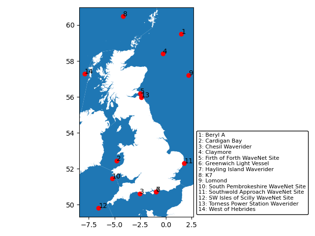
Key Points
Geopandas is the key module to help deal with geospatial data.
Using Geopandas and Geoplot we can create publication / web-ready maps.